01 CNN (컨볼루션 신경망)
02 유명인사의 얼굴 데이터 분류하기
-01 이미지 분석 - pca + knn (얼굴 데이터)
-02 이미지 분석 - ANN(3차원 학습 불가) (얼굴 데이터)
-03 이미지 분석 - CNN(3차원 학습 가능) (얼굴 데이터)
-04 새로운 얼굴 사진 예측 함수
-05 사전학습 모델(EfficientNetB0) + 얼굴 데이터 전이학습
03 쇼핑몰 후기 감성 분석
01 CNN (컨볼루션 신경망)
- 심층신경망에 컨볼루션 망을 추가한 신경망
- 컨볼루션 망에서 이미지의 정교한 특징을 추출
- 마스크(=필터=윈도우)에 의해서 재추출된 신호
- hyper parameter : 컨볼루션층 수, 마스크 수, 마스크 사이즈
- parameter : 각 마스크 가중치
- 풀링(=서브샘플링) : 기존 이미지 신호 중 일부를 추출하여 보다 단순한 맵으로 결정 -> 과적합 해소
pool_size는 (2,2), (3,3), (4,4) 등을 사용 <- hyper marameter
pool에 의해 추출되는 신호는 주로 최댓값(max pooling), 평균값(average pooling) 등
- Dropout : 의도적으로 특정 층의 중요하지 않은 노드(뉴런=Unit)를 꺼버리는 기법 -> 과적합 해소
size는 보통 0.5, 0.25 등을 주로 사용 <- hyper parameter
02 유명인사의 얼굴 데이터 분류하기
-01 이미지 분석 - pca + knn (얼굴 데이터)
1) 데이터 로딩
from sklearn.datasets import fetch_lfw_people
import numpy as np
people = fetch_lfw_people(min_faces_per_person=50, resize=0.7) # 스케일링 된 데이터
X = people['data']
X_images = people['images']
y = people['target']
yname = people['target_names']
n_classes = len(yname)
# 데이터 확인
import matplotlib.pyplot as plt
X_images[0].shape
X_images[0].shape
Out[159]: (87, 65)
plt.imshow(X_images[1], cmap='gray')
yname[y[1]]
2) 데이터 분리
from sklearn.model_selection import train_test_split
train_x, test_x, train_y, test_y = train_test_split(X, y, random_state=0, stratify=y)
3) 모델링
# 1) knn
from sklearn.neighbors import KNeighborsClassifier
m_knn = KNeighborsClassifier()
m_knn.fit(train_x, train_y)
m_knn.score(train_x, train_y) # 0.6863
m_knn.score(test_x, test_y) # 0.4974
# 2) pca + knn
from sklearn.decomposition import PCA
from sklearn.pipeline import make_pipeline
pipe = make_pipeline(PCA(100), KNeighborsClassifier(5))
pipe.fit(train_x, train_y)
pipe.score(train_x, train_y) # 0.6965
pipe.score(test_x, test_y) # 0.4974
-02 이미지 분석 - ANN(3차원 학습 불가) (얼굴 데이터)
1) 데이터 로딩
from sklearn.datasets import fetch_lfw_people
import numpy as np
people = fetch_lfw_people(min_faces_per_person=50, resize=0.7)
X = people['data']
X_images = people['images']
y = people['target']
yname = people['target_names']
n_classes = len(yname)
2) 데이터 분리
from sklearn.model_selection import train_test_split
train_x, test_x, train_y, test_y = train_test_split(X, y, random_state=0, stratify=y)
# 원핫 인코딩
import pandas as pd
train_y10 = pd.get_dummies(train_y, prefix='Y').astype(int).values
test_y10 = pd.get_dummies(test_y, prefix='Y').astype(int).values
3) 모델링
# 1) seed 고정
import tensorflow as tf
seed = 0
np.random.seed(seed)
tf.random.set_seed(seed)
# 2) 모델 정의
from tensorflow.keras.layers import Input, Dense
from keras import Sequential
model = Sequential()
model.add(Input(shape=(train_x.shape[1], )))
model.add(Dense(392, activation='relu'))
model.add(Dense(196, activation='relu'))
model.add(Dense(98, activation='relu'))
model.add(Dense(n_classes, activation='softmax'))
# 3) 오차함수, 최적화 결정
model.compile(optimizer='adam', loss='categorical_crossentropy', metrics=['accuracy'])
# 4) early stopping rule
from tensorflow.keras.callbacks import EarlyStopping
es = EarlyStopping(monitor='val_loss', patience=10, restore_best_weights=True)
# 5) 학습
hist = model.fit(train_x, train_y10, validation_split=0.25,
batch_size=10, epochs=50000, callbacks=[es])
# 6) 평가
model.evaluate(train_x, train_y10)[1] # 0.6871
model.evaluate(test_x, test_y10)[1] # 0.5948
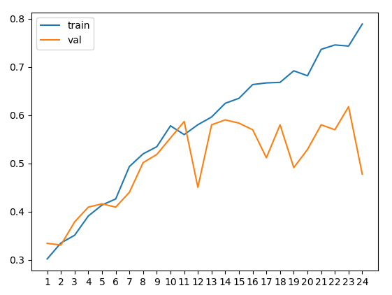
acc = hist.history['accuracy']
plt.plot(range(1, len(acc)+1), hist.history['accuracy'], label='train')
plt.plot(range(1, len(acc)+1), hist.history['val_accuracy'], label='val')
plt.legend()
plt.xticks(range(1, len(acc)+1))
-03 이미지 분석 - CNN(3차원 학습 가능) (얼굴 데이터)
1) 데이터 로딩
from sklearn.datasets import fetch_lfw_people
import numpy as np
people = fetch_lfw_people(min_faces_per_person=50, resize=0.7)
X = people['data']
X_images = people['images']
y = people['target']
yname = people['target_names']
n_classes = len(yname)
h, w = X_images.shape[1], X_images.shape[2]
2) 데이터 분리 및 변환
from sklearn.model_selection import train_test_split
train_x, test_x, train_y, test_y = train_test_split(X_images, y, random_state=0, stratify=y)
# ** Conv2D 층은 (높이, 너비, 채널) 형태 요구 (흑백 -> 채널:1)
train_x = train_x.reshape((train_x.shape[0], h, w, 1))
test_x = test_x.reshape((test_x.shape[0], h, w, 1))
import pandas as pd
train_y10 = pd.get_dummies(train_y).astype(int).values
test_y10 = pd.get_dummies(test_y).astype(int).values
3) 모델링
# 1) seed 고정
import tensorflow as tf
seed = 0
np.random.seed(seed)
tf.random.set_seed(seed)
# 2) 모델 정의
from tensorflow.keras.layers import Input, Dense, Conv2D, Dropout, Flatten, MaxPooling2D
from keras import Sequential
model = Sequential()
model.add(Input(shape=(h, w, 1)))
model.add(Conv2D(32, kernel_size=(2, 2), activation='relu'))
model.add(Conv2D(32, kernel_size=(2, 2), activation='relu'))
model.add(MaxPooling2D((2, 2)))
model.add(Flatten())
model.add(Dense(128, activation='relu'))
model.add(Dropout(0.5))
model.add(Dense(n_classes, activation='softmax'))
# 3) compile
model.compile('adam', loss='categorical_crossentropy', metrics=['accuracy'])
# 4) 정지규칙
from tensorflow.keras.callbacks import EarlyStopping
es = EarlyStopping(monitor='val_loss', patience=10, restore_best_weights=True)
# 5) 학습
hist = model.fit(train_x, train_y10, validation_split=0.25,
batch_size=10, epochs=50000, callbacks=[es])
# 6) 평가
model.evaluate(train_x, train_y10)[1] # 0.9393
model.evaluate(test_x, test_y10)[1] # 0.7051
acc = hist.history['accuracy']
plt.plot(range(1, len(acc)+1), hist.history['accuracy'], label='train')
plt.plot(range(1, len(acc)+1), hist.history['val_accuracy'], label='val')
plt.legend()
plt.xticks(range(1, len(acc)+1))

-04 새로운 얼굴 사진 예측 함수
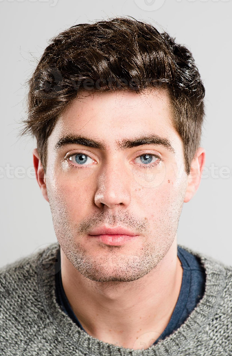
# 데이터 경로에 다음 사진을 넣어준다.
from PIL import Image
import numpy as np
import matplotlib.pyplot as plt
plt.rcParams['font.family'] = 'Malgun Gothic' # Windows
plt.rcParams['axes.unicode_minus'] = False # 마이너스 기호 깨짐 방지
def f_predict_face(img_path, model, h, w, yname, X_images, y):
# 1) 이미지 로딩 및 흑백 변환
img = Image.open(img_path).convert('L') # 흑백(그레이스케일) 변환
# 2) 크기 맞추기 (학습 데이터와 동일한 h, w)
img = img.resize((w, h)) # PIL은 (width, height) 순서
# 3) 배열 변환 및 스케일링 (0~255 -> 0~1)
img_arr = np.array(img) / 255.0
# 4) CNN 입력 형태로 변환 (1, h, w, 1)
img_input = img_arr.reshape((1, h, w, 1))
# 5) 예측
pred = model.predict(img_input)
pred_class = pred.argmax(axis=1)[0]
pred_name = yname[pred_class]
pred_prob = pred[0][pred_class]
print(f"예측 인물: {pred_name}, 확률: {pred_prob:.4f}")
# 6) 입력 사진 vs 예측된 클래스의 실제 사진 비교 출력
real_img = X_images[y == pred_class][0] # 예측 클래스의 실제 이미지 하나 추출
fig, ax = plt.subplots(1, 2)
ax[0].imshow(img_arr, cmap='gray')
ax[0].set_title('입력 사진')
ax[0].axis('off')
ax[1].imshow(real_img, cmap='gray')
ax[1].set_title(f'예측: {pred_name}')
ax[1].axis('off')
# 사용 예시
f_predict_face('image_sample.jpg', model, h, w, yname, X_images, y)

f_predict_face('image_sample.jpg', model, h, w, yname, X_images, y)
1/1 ━━━━━━━━━━━━━━━━━━━━ 0s 60ms/step
예측 인물: Junichiro Koizumi, 확률: 0.7375
-05 사전학습 모델(EfficientNetB0) + 얼굴 데이터 전이학습
1) 데이터 로딩 (컬러로 로드해야 사전학습 모델 입력에 맞음)
from sklearn.datasets import fetch_lfw_people
import numpy as np
people = fetch_lfw_people(min_faces_per_person=50, resize=0.7, color=True)
X_images = people['images'] # (n, h, w, 3)
y = people['target']
yname = people['target_names']
n_classes = len(yname)
h, w = X_images.shape[1], X_images.shape[2]
2) 데이터 분리
from sklearn.model_selection import train_test_split
train_x, test_x, train_y, test_y = train_test_split(X_images, y, random_state=0, stratify=y)
3) 사전학습 모델 입력 크기(224x224)로 리사이즈
import tensorflow as tf
def resize_batch(x, size=(224, 224)):
x = tf.image.resize(x, size)
return x.numpy()
train_x_rs = resize_batch(train_x)
test_x_rs = resize_batch(test_x)
# EfficientNet은 0~255 입력을 받아 내부적으로 전처리하므로 /255 하지 않음
# (fetch_lfw_people은 0~1로 스케일링되어 있으므로 되돌려줌)
train_x_rs = train_x_rs * 255
test_x_rs = test_x_rs * 255
# 원핫 인코딩
import pandas as pd
train_y10 = pd.get_dummies(train_y).astype(int).values
test_y10 = pd.get_dummies(test_y).astype(int).values
4) 사전학습 모델 로딩 (특성 추출기로 사용, 가중치 고정)
from tensorflow.keras.applications import EfficientNetB0
from tensorflow.keras.layers import Input, Dense, Dropout, GlobalAveragePooling2D
from tensorflow.keras.models import Model
base_model = EfficientNetB0(include_top=False, # ImageNet 1000개 클래스용 마지막 분류층을 빼고, 출력층을 새로 붙이겠다는 옵션
weights='imagenet', # 이미지 분류 연구용으로 만든 대규모 데이터셋(1,000개 클래스, 약 120만 장)
input_shape=(224, 224, 3)) # ImageNet 학습 크기이므로 사용 권장(변경가능)
base_model.trainable = False # 사전학습 가중치 고정 (feature extractor로만 사용)
# 모델 생성(base_model 자체가 이미 완성된 하나의 모델이므로 Sequential 방식 사용 불가 -> Functional API 방식 사용)
# Functional API : 각 층을 함수처럼 다루면서 입력과 출력을 직접 연결하는 방식
inputs = Input(shape=(224, 224, 3))
x = base_model(inputs, training=False)
x = GlobalAveragePooling2D()(x)
x = Dense(128, activation='relu')(x)
x = Dropout(0.5)(x)
outputs = Dense(n_classes, activation='softmax')(x) # 얼굴 데이터 출력 층 연결
model = Model(inputs, outputs)
model.compile('adam', loss='categorical_crossentropy', metrics=['accuracy'])
5) 학습
from tensorflow.keras.callbacks import EarlyStopping
es = EarlyStopping(monitor='val_loss', patience=5, restore_best_weights=True)
hist = model.fit(train_x_rs, train_y10, validation_split=0.25,
batch_size=16, epochs=50, callbacks=[es])
6) 평가
model.evaluate(train_x_rs, train_y10)[1] # 0.9820
model.evaluate(test_x_rs, test_y10)[1] # 0.9102
03 쇼핑몰 후기 감성 분석
import pandas as pd
df = pd.read_table('shopping_ratings_total.txt', names = ['ratings', 'reviews'])
df.head()
df.head()
Out[328]:
   ratings                                            reviews
0        5                                            배공빠르고 굿
1        2                      택배가 엉망이네용 저희집 밑에층에 말도없이 놔두고가고
2        5  아주좋아요 바지 정말 좋아서2개 더 구매했어요 이가격에 대박입니다. 바느질이 조금 ...
3        2  선물용으로 빨리 받아서 전달했어야 하는 상품이었는데 머그컵만 와서 당황했습니다. 전...
4        5                  민트색상 예뻐요. 옆 손잡이는 거는 용도로도 사용되네요 ㅎㅎ
...
df.shape
df.shape
Out[329]: (200000, 2)
2) target 변수 변환 (평점 -> 이진데이터)
import numpy as np
np.unique(df['ratings'])
np.unique(df['ratings'])
Out[6]: array([1, 2, 4, 5])
3) 샘플링
# 실제 분석 과정에서는 생략한다.
# 금일 실습에서는 20만건 학습이 불가능한 상황이기 때문에 3만건만 우선 랜덤샘플링을 진행한다.
df = df.sample(n=30000, random_state=0).reset_index(drop=True) # 랜덤 샘플링이기 때문에 index를 초기화한다.
4) 데이터 분리 (train/test)
from sklearn.model_selection import train_test_split
train_test_aplit(df['reviews'], df['ratings'], random_state=0, stratify=df['ratings'])
5) 전처리 (정제 -> 형태소 분석)
# pip install konlpy
import konlpy.tag
Okt = konlpy.tag.Okt() # RuntimeError: Java versioin too old. Java 9 or later is required
# cmd에서 java -version
# ** java 최신버전 설치
# https://www.oracle.com/java/technologies/downloads/#jdk26-windows
# 설치 후 명령 프롬포트는 다시 실행한 다음에 버전확인이 적용된다.
# 이후 path 등록을 진행해야 한다. (시스템 환경 변수 편집 - 환경 변수 - path - 다운로드 받은 C:\Program Files\Java\jdk-26.0.2\bin 추가 후 확인)
'아이티윌_데이터 분석 55기 > 강의내용_딥러닝' 카테고리의 다른 글
| #5 5일차_감성 분석 (나이브베이즈, RNN) (0) | 2026.07.29 |
|---|---|
| #3 3일차_ANN(다중 분류), 이미지 분석(PCA+KNN, ANN, CNN) (0) | 2026.07.27 |
| #2 2일차_인공신경망의 구조, 실습 (0) | 2026.07.24 |
| #1 1일차_tensorflow, keras 설치하기 (0) | 2026.07.23 |