01 클래스 불균등 처리
-01 언더샘플링
-02 오버샘플링
-03 가중치 조절
-04 임계값 이동
01 클래스 불균등 처리
-01 언더샘플링
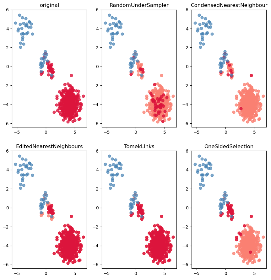
1) RandomUnderSampler
- 다수 클래스 데이터를 랜덤하게 선택하여 제거
- 다수 : 소수 비율이 정확히 1 : 1이 됨
- 중요한 데이터의 손실 발생 위험이 존재 (가장 위험한 방법)
2) CondensedNearestNeighbour
- 뭉쳐져있는 다수 클래스를 중복으로 가정하고 제거 -> 결정결계와 먼 다수클래스를 제거
- 다수 클래스 데이터에서 랜덤하게 데이터를 선택하며, k개의 가장 가까운 이웃을 확인 후, 그 이웃이 다수클래스 (같은편)이면 제거
3) EditedNearestNeighbours
- 결정경계 근처에 있는 다수클래스 일부를 제거 -> 좀 더 단순한 결정 경계가 만들어짐
- 다수 클래스 데이터에서 랜덤하게 데이터 선택, k개의 가장 가까운 이웃을 확인, 그 이웃이 소수클래스 (다른편)이면 제거
4) TomekLinks
- TomekLink : 소수, 다수 클래스 각각 관측치 기준 가장 가까운 이웃이 서로가 되는 한 쌍
- TomekLink 쌍 중에서 다수 클래스를 제거하는 방식
- 결정경계가 복잡하지 않은 경우는 다수 클래스가 제거되지 않을 수 있음
5) OneSidedSelection (OSS)
- TomekLink + CNN
[ 예제 - 각 언더샘플링 기법 비교 ]
# 1. 데이터 로딩
import pandas as pd
df = pd.read_csv('undersampling_data.csv')
X = df[['x1','x2']]
y = df['y']
# 각 클래스 도수 / 비율 확인
y.value_counts()
y.value_counts(normalize = True) # 0:다수클래스 (91.6%), 1: 소수클래스(8.4%)
y.value_counts(normalize = True)
Out[138]:
y
0    0.916045
1    0.083955
Name: proportion, dtype: float64
# 2. 언더샘플링
from imblearn.under_sampling import RandomUnderSampler, CondensedNearestNeighbour, EditedNearestNeighbours, TomekLinks, OneSidedSelection
import imblearn.under_sampling
dir(imblearn.under_sampling)
m1 = RandomUnderSampler()
m2 = CondensedNearestNeighbour()
m3 = EditedNearestNeighbours()
m4 = TomekLinks()
m5 = OneSidedSelection()
X1, y1 = m1.fit_resample(X,y)
print(pd.Series(y1).value_counts(normalize = True))
print(pd.Series(y1).value_counts(normalize = True))
y
0    0.5
1    0.5
Name: proportion, dtype: float64
X2, y2 = m2.fit_resample(X,y)
print(pd.Series(y2).value_counts(normalize = True))
print(pd.Series(y2).value_counts(normalize = True))
y
1    0.803571
0    0.196429
Name: proportion, dtype: float64
X3, y3 = m3.fit_resample(X,y)
print(pd.Series(y3).value_counts(normalize = True))
print(pd.Series(y3).value_counts(normalize = True))
y
0    0.913958
1    0.086042
Name: proportion, dtype: float64
X4, y4 = m4.fit_resample(X,y)
print(pd.Series(y4).value_counts(normalize = True))
print(pd.Series(y4).value_counts(normalize = True))
y
0    0.915254
1    0.084746
Name: proportion, dtype: float64
X5, y5 = m5.fit_resample(X,y)
print(pd.Series(y5).value_counts(normalize = True))
print(pd.Series(y5).value_counts(normalize = True))
y
1    0.511364
0    0.488636
Name: proportion, dtype: float64
# 3. 시각화
import matplotlib.pyplot as plt
fig, ax = plt.subplots(2,3)
# 기본 산점도
ax[0,0].scatter(X[y==0,0], X[y==0,1], c='crimson', s=40, alpha = 0.8)
ax[0,0].scatter(X[y==1,0], X[y==1,1], c='steelblue', s=40, alpha = 0.7)
ax[0,0].set_title('original')
# RandomUnderSampler
ax[0,1].scatter(X[y==0,0], X[y==0,1], c='salmon', s=40, alpha = 0.8)
ax[0,1].scatter(X1[y1==0,0], X1[y1==0,1], c='crimson', s=40, alpha = 0.8)
ax[0,1].scatter(X1[y1==1,0], X1[y1==1,1], c='steelblue', s=40, alpha = 0.7)
ax[0,1].set_title('RandomUnderSampler')
# CondensedNearestNeighbour
ax[0,2].scatter(X[y==0,0], X[y==0,1], c='salmon', s=40, alpha = 0.8)
ax[0,2].scatter(X2[y2==0,0], X2[y2==0,1], c='crimson', s=40, alpha = 0.8)
ax[0,2].scatter(X2[y2==1,0], X2[y2==1,1], c='steelblue', s=40, alpha = 0.7)
ax[0,2].set_title('CondensedNearestNeighbour')
# EditedNearestNeighbours
ax[1,0].scatter(X[y==0,0], X[y==0,1], c='salmon', s=40, alpha = 0.8)
ax[1,0].scatter(X3[y3==0,0], X3[y3==0,1], c='crimson', s=40, alpha = 0.8)
ax[1,0].scatter(X3[y3==1,0], X3[y3==1,1], c='steelblue', s=40, alpha = 0.7)
ax[1,0].set_title('EditedNearestNeighbours')
# TomekLinks
ax[1,1].scatter(X[y==0,0], X[y==0,1], c='salmon', s=40, alpha = 0.8)
ax[1,1].scatter(X4[y4==0,0], X4[y4==0,1], c='crimson', s=40, alpha = 0.8)
ax[1,1].scatter(X4[y4==1,0], X4[y4==1,1], c='steelblue', s=40, alpha = 0.7)
ax[1,1].set_title('TomekLinks')
# OneSidedSelection
ax[1,2].scatter(X[y==0,0], X[y==0,1], c='salmon', s=40, alpha = 0.8)
ax[1,2].scatter(X5[y5==0,0], X5[y5==0,1], c='crimson', s=40, alpha = 0.8)
ax[1,2].scatter(X5[y5==1,0], X5[y5==1,1], c='steelblue', s=40, alpha = 0.7)
ax[1,2].set_title('OneSidedSelection')
-02 오버샘플링
소수 클래스 관측치를 다수 클래스 관측치수와 유사하게 임의로 생성하여 균등하게 맞추는 샘플링 기법
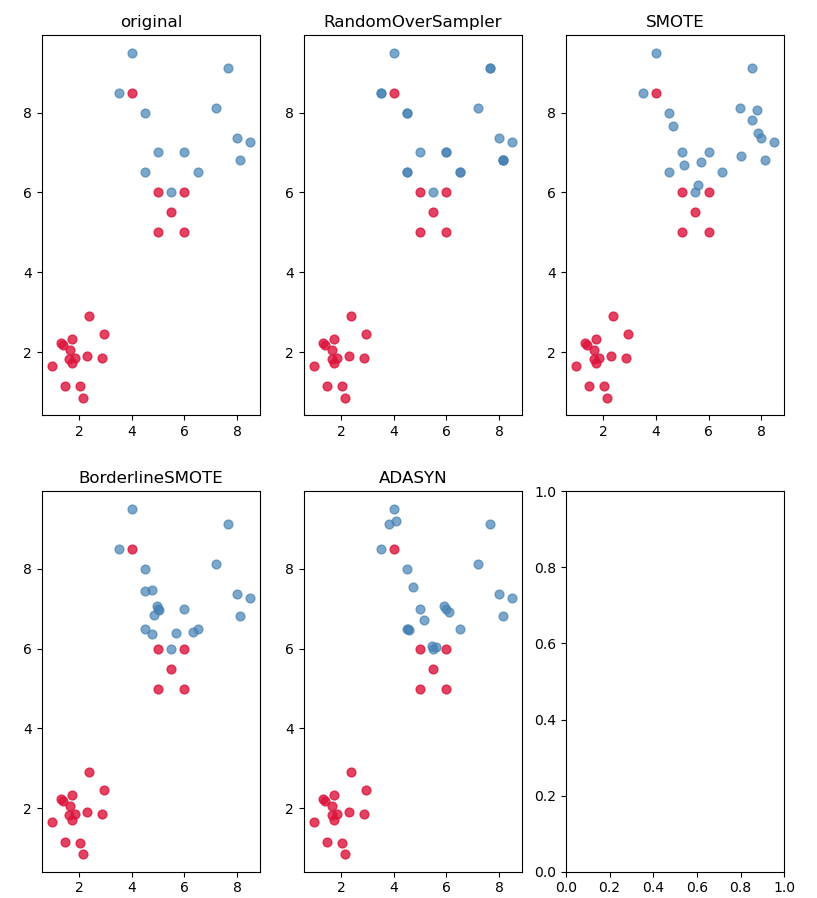
1) RandomOverSampler
- 소수 클래스 관측치를 동일하게 재생성 -> 데이터의 중복 발생
- 1:1의 비율로 데이터를 샘플하기 때문에 빈도를 잘 맞추어준다.
2) SMOTE
- 이웃들 중 하나를 선택하여 이웃과의 사이에 새로운 데이터를 생성
- 임의의 소수 클래스 데이터 선택, k개의 가장 가까운 이웃 데이터 확인, 그 중 랜덤하게 선택된 다수클래스와의 사이에 소수클래스 생성
- 결정경계 근처가 아닌 공간에도 소수 클래스 데이터가 생성될 수 있다. = 소수와 다수가 밀집한 공간이 아님에도 불구하고 소수클래스를 배치하면 결정경계가 이동할 수도 있다.
3) BorderlineSMOTE
- SMOTE와 결정경계가 아닌 지역에도 소수클래스를 생성하는 단점을 보완
- 소스클래스를 다음의 세 집단으로 구분하여 위험 지역에만 소수 클래스를 생성
> 위험 : 이웃 중 다수가 다수 클래스
> 안전 : 이웃 중 소수가 다수 클래스
> 심플 : 이웃 중 다수 클래스가 아예 없는 경우
- 임의의 소수 클래스 데이터 선택, k개의 가장 가까운 이웃 데이터 확인, 그 중 랜덤하게 선택된 다수 클래스와의 사이에 소수클래스 생성
- 결정경계 근처에만 소수 클래스 데이터가 생성됨
4) ADASYN
- 인근 다수클래스 비율 확인 -> 비율을 반영하여 소수클래스 생성
# 1. 데이터 로딩
import pandas as pd
df = pd.read_csv('oversampling_data.csv')
X = df[['x1','x2']].values
y = df['y'].values
# 각 클래스 도수 / 비율 확인
pd.Series(y).value_counts()
pd.Series(y).value_counts(normalize = True) # 0 : 다수클래스 (62%), 1 : 소수클래스 (38%)
# 2. 오버샘플링
from imblearn.over_sampling import RandomOverSampler, SMOTE, BorderlineSMOTE, ADASYN
import imblearn.over_sampling
m1 = RandomOverSampler(random_state=0)
m2 = SMOTE(random_state=0, k_neighbors=5)
m3 = BorderlineSMOTE(random_state=0, k_neighbors=5)
m4 = ADASYN(random_state=0, n_neighbors=5)
X1, y1 = m1.fit_resample(X,y)
print(pd.Series(y1).value_counts())
X2, y2 = m2.fit_resample(X,y)
print(pd.Series(y2).value_counts())
X3, y3 = m3.fit_resample(X,y)
print(pd.Series(y3).value_counts())
X4, y4 = m4.fit_resample(X,y)
print(pd.Series(y4).value_counts())
# 3. 시각화
import matplotlib.pyplot as plt
fig, ax = plt.subplots(2,3)
# 기본 산점도
ax[0,0].scatter(X[y==0,0], X[y==0,1], c='crimson', s=40, alpha = 0.8)
ax[0,0].scatter(X[y==1,0], X[y==1,1], c='steelblue', s=40, alpha = 0.7)
ax[0,0].set_title('original')
# RandomOverSampler
ax[0,1].scatter(X1[y1==0,0], X1[y1==0,1], c='crimson', s=40, alpha = 0.8)
ax[0,1].scatter(X1[y1==1,0], X1[y1==1,1], c='steelblue', s=40, alpha = 0.7)
ax[0,1].set_title('RandomOverSampler')
# SMOTE
ax[0,2].scatter(X2[y2==0,0], X2[y2==0,1], c='crimson', s=40, alpha = 0.8)
ax[0,2].scatter(X2[y2==1,0], X2[y2==1,1], c='steelblue', s=40, alpha = 0.7)
ax[0,2].set_title('SMOTE')
# BorderlineSMOTE
ax[1,0].scatter(X3[y3==0,0], X3[y3==0,1], c='crimson', s=40, alpha = 0.8)
ax[1,0].scatter(X3[y3==1,0], X3[y3==1,1], c='steelblue', s=40, alpha = 0.7)
ax[1,0].set_title('BorderlineSMOTE')
# ADASYN
ax[1,1].scatter(X4[y4==0,0], X4[y4==0,1], c='crimson', s=40, alpha = 0.8)
ax[1,1].scatter(X4[y4==1,0], X4[y4==1,1], c='steelblue', s=40, alpha = 0.7)
ax[1,1].set_title('ADASYN')
-03 가중치 조절
모델 학습 시 소수 클래스 예측 실패에 대해 패널티를 부여하는 기법
대부분 분류 모델이 가중치 조절 옵션 존재
가장 단순하게 사용 가능한 기법 (가장 먼저 고려)
-04 임계값 이동
모델의 예측력을 향상시키는 직접적인 방법은 아님
소수클래스 예측 실패를 막기 위해 소수클래스일 확률이 조금이라도 있으면 소수클래스로 예측해버리는 기법
이진 클래스) 소수 클래스 확률이 0.5 이상이면 소수클래스로 예측하는데, 이 임계값을 낮춤으로써 소수 클래스가 더 많이 나올 수 있도록 조절하는 방식
다수 클래스) 각 클래스별 확률을 각 클래스별 도수로 나눈 값으로 클래스 예측을 수행하는 방식
1) 클래스 2개
ex ) 소수클래스 (y=1), 다수클래스 (Y=0)
* 기본 클래스 결정 방식 : 소수클래스 확률 기준으로 0.5 이상 여부 확인
P(Y=1) >= 0.5 -> Y는 1로 결정
P(Y=0) < 0.5 -> Y는 0으로 결정
* 소수 클래스 예측률을 올리려면? 소수클래스 예측 결과를 더 많이 얻을 수 있도록 임계값을 변경
P(Y=1) >= 0.3 -> Y는 1로 결정 (임계값이 0.5일때보다 소수클래스가 더 많아짐)
P(Y=1) < 0.3 -> Y는 0으로 결정
2) 클래스 3개 이상
각 클래스의 확률을 각 클래스 빈도 / 비율로 나누어서
다수클래스 확률을 보다 작게, 소수클래스 확률을 보다 크게 만드는 방식
0.7 0.2 0.1 <---비율
P(Y=0) P(Y=1) P(Y=2)
0.1 0.2 0.7 -> 2
0.5 0.2 0.3 -> 0
활성화 함수는 softmax : 각 비율을 기준으로 확률이 가장 높은 집단을 선택하는 방식
[ 연습문제 - 클래스 불균등 조치 ]
**** 추후 추가
02 회귀 분석
Y가 존재하는 지도학습 형태
Y가 수치형인 경우의 분석
** 파이썬에서의 회귀분석 모델링 방식
-01 sklearn 선형회귀모델 사용
- 코드 구현이 간편 (상수항 추가 기본)
- score 메서드로 평가점수 쉽게 확인 가능
(분류에서는 accuracy, 회귀에서는 R2 (수정계수 아님!))
- 유의성 검정 결과 확인 불가
-02 statsmodels 선형회귀모델 사용
- 코드 구현 비교적 불편 (상수항 추가 필수)
- 유의성 검정 결과 확인 가능 (p-value)
- (빅분기) 작업 3유형에서 회귀모형에서의 특정 변수 p-value를 확인하라는 경우가 있어서 외우는 것이 좋다.
-03 sklearn 분류 알고리즘을 사용한 회귀 적합 (SVR, DTR, RFR 등)
- 코드 구현 간편 (상수항 추가 기본)
- score 멤서드(R2)로 평가점수 쉽게 확인 가능
- 유의성 검정 결과 확인 불가
- 여러 모형의 장점을 활용한 회귀 적합 가능
- (빅분기) 작업 2유형을 위해서 외우는 것이 좋다.
# ** 회귀 알고리즘
사전에 등분산성을 검정한다.
두 집단의 분산이 같을 때와 다를 때 검정통계량을 계산하는 수식이 달라진다.
정규성 가정 -> F 가정 (이론적인 가정으로 현업에서는 잘 사용하지 않는다.)
레빈 테스트 등을 더 많이 사용한다. (정규성 가정을 하지 않는다.)
1) 전통회귀 (릿지, 라쏘, 엘라스틱넷)
- 여러 통계적 가정 피룡
- 변수 선택 중요
- 다중공선성 확인 필수
- 유의성 검정 결과
- 인과 관계 파악 가능
- 릿지, 라쏘 엘라스틱넷은 패널티 모형
각각의 회귀계수가 너무 커지거나 과적합이 되는 것을 막아준다.
때로는 회귀계수를 0으로 만들어준다. (해당 변수를 제거하는 효과가 있다.)
2) 분류 알고리즘 회귀 적합 (SVM, RF, KNN 등)
- 예측력 우수
- 변수선택이 필수가 아님
- 이상치에 민감하지 않을 수 있음
- 유의성 검정 결과 제시 x
- 인과 관계 파악 불가
[ 예제 - 보스턴 주택가격 예측 ]
# 1. 데이터 로딩
df = pd.read_csv('boston.csv')
X = df.drop(columns = 'medv')
y = df['medv']
# 2. 데이터 분리
from sklearn.model_selection import train_test_split
train_x, test_x, train_y, test_y = train_test_split(X, y, random_state = 0)
# 3. 모델링
# 1) sklearn 선형회귀
from sklearn.linear_model import LinearRegression
m_lr = LinearRegression()
m_lr.fit(train_x, train_y)
m_lr.score(train_x, train_y) # 0.7698
m_lr.score(test_x, test_y) # 0.6355
# 예측
pre_tr_lr = m_lr.predict(train_x)
pre_te_lr = m_lr.predict(test_x)
# 2) statsmodels
import statsmodels.api as sm
# 상수항 추가
train_x_const = sm.add_constant(train_x)
# 회귀모형 적합
m_lr2 = sm.OLS(train_y, train_x_const).fit()
# 결과확인
m_lr2.summary() # 유의성 검정 결과 (R2 = 0.770)
# H0 : 모형이 적합하지 않다.
# H1 : 모형이 적합하다.
# Prob (F-statistic): 9.85e-108
# 해당 모형은 적합하다.
m_lr2.summary()
Out[268]:
<class 'statsmodels.iolib.summary.Summary'>
"""
                            OLS Regression Results
==============================================================================
Dep. Variable:                   medv   R-squared:                       0.770
Model:                            OLS   Adj. R-squared:                  0.762
Method:                 Least Squares   F-statistic:                     93.87
Date:                Mon, 15 Jun 2026   Prob (F-statistic):          9.85e-108
Time:                        16:04:56   Log-Likelihood:                -1102.0
No. Observations:                 379   AIC:                             2232.
Df Residuals:                     365   BIC:                             2287.
Df Model:                          13
Covariance Type:            nonrobust
==============================================================================
                 coef    std err          t      P>|t|      [0.025      0.975]
------------------------------------------------------------------------------
const         36.9333      5.682      6.500      0.000      25.759      48.107
crim          -0.1177      0.037     -3.143      0.002      -0.191      -0.044
zn             0.0440      0.015      2.933      0.004       0.015       0.074
indus         -0.0058      0.067     -0.086      0.931      -0.137       0.125
chas           2.3934      0.962      2.488      0.013       0.502       4.285
nox          -15.5894      4.331     -3.600      0.000     -24.106      -7.073
rm             3.7690      0.472      7.981      0.000       2.840       4.698
age           -0.0070      0.015     -0.472      0.637      -0.036       0.022
dis           -1.4350      0.224     -6.401      0.000      -1.876      -0.994
rad            0.2401      0.073      3.301      0.001       0.097       0.383
tax           -0.0113      0.004     -2.779      0.006      -0.019      -0.003
ptratio       -0.9855      0.145     -6.793      0.000      -1.271      -0.700
black          0.0084      0.003      2.782      0.006       0.002       0.014
lstat         -0.4991      0.058     -8.667      0.000      -0.612      -0.386
==============================================================================
Omnibus:                      141.715   Durbin-Watson:                   2.025
Prob(Omnibus):                  0.000   Jarque-Bera (JB):              665.545
Skew:                           1.549   Prob(JB):                    3.01e-145
Kurtosis:                       8.705   Cond. No.                     1.53e+04
==============================================================================

Notes:
[1] Standard Errors assume that the covariance matrix of the errors is correctly specified.
[2] The condition number is large, 1.53e+04. This might indicate that there are
strong multicollinearity or other numerical problems.
"""
결론)
1. 모형의 유의성 검정 결과 확인 (F검정)
H0 : 모형이 유의하지 않다.
H1 : 모형이 유의하다.
dir(m_lr2)
m_lr2.f_pvalue
m_lr2.f_pvalue
Out[271]: np.float64(9.846025348751037e-108)
< 0.05이므로 영가설 기각 -> 모형이 유의함
2. 독립변수 유의성 검정 결과 확인 (T검정)
H0 : 각 회귀계수가 0이다.
H1 : 각 회귀계수가 0이 아니다.
m_lr2.pvalues
m_lr2.pvalues
Out[273]:
const      2.645323e-10
crim       1.809488e-03
zn         3.572238e-03
indus      9.311837e-01
chas       1.327649e-02
nox        3.624962e-04
rm         1.901692e-14
age        6.373763e-01
dis        4.734867e-10
rad        1.058885e-03
tax        5.732066e-03
ptratio    4.479130e-11
black      5.678867e-03
lstat      1.461667e-16
dtype: float64
# 유의하지 않은 변수 확인
m_lr2.pvalues[m_lr2.pvalues > 0.05]
m_lr2.pvalues[m_lr2.pvalues > 0.05]
Out[274]:
indus    0.931184
age      0.637376
dtype: float64
# 가장 유의한 변수 이름
m_lr2.pvalues.drop('const').idxmin()
m_lr2.pvalues.drop('const').idxmin()
Out[276]: 'lstat'
# 가장 유의한 변수의 회귀 계수 확인
m_lr2.params['lstat']
m_lr2.params['lstat']
Out[279]: np.float64(-0.4991167973261213)
# 3. 모형의 설명력
m_lr2.rsquared # 결정계수
m_lr2.rsquared_adj # 수정결정계수 (독립변수의 수가 다른 모형 비교시 사용)
m_lr2.rsquared     # 결정계수
Out[281]: np.float64(0.7697699488741148)

m_lr2.rsquared_adj # 수정결정계수 (독립변수의 수가 다른 모형 비교시 사용)
Out[282]: np.float64(0.7615699744504532)
# 3) 기타 분류모형 회귀 적합
from sklearn.svm import SVR
from sklearn.ensemble import RandomForestClassifier
'아이티윌_데이터 분석 55기 > 강의내용 필기_분석(Python)' 카테고리의 다른 글
| #12 12일차_군집분석, 연관분석 (0) | 2026.06.19 |
|---|---|
| #10 회귀모형과 패널티 모형, 부스팅 이론 (0) | 2026.06.18 |
| #7 7일차_독립성 검정, 적합도 검정, 클래스 불균등 처리 (0) | 2026.06.11 |
| #6 교호작용 및 효과 검증 (0) | 2026.06.09 |
| #5 5일차_데이터 분석 과정, 로지스틱 회귀, 교호작용 (0) | 2026.06.08 |