[ 과제5. 교호작용 효과 검증 ]
# 1. 데이터 로딩 및 설명
import pandas as pd
pd.set_option('display.max_column', None)
df = pd.read_csv('telecom_churn.csv')
# X, y 분리 / 노이즈 변수 제거
X = df.drop(columns=['churn','phone number'])
y = df['churn']
# 변수 추가
X['total minutes'] = X.loc[:, X.columns.str.contains('minutes')].sum(axis=1) # 총 통화시간
X['total calls'] = X.loc[:, X.columns.str.contains('calls')].sum(axis=1) # 총 통화건수
X['total charge'] = X.loc[:, X.columns.str.contains('charge')].sum(axis=1) # 총 요금
# 노이즈 변수 제거
X = X.drop(columns=['state','area code','total eve calls','total calls'])
# 2. 라벨 인코딩
obj_cols = X.select_dtypes(include='object').columns # 문자형 컬럼만 선택 -> 라벨인코딩
num_cols = X.select_dtypes(exclude='object').columns # 숫자형 컬럼만 선택 -> 스케일링
from sklearn.preprocessing import LabelEncoder
for colname in obj_cols:
m_ec = LabelEncoder()
X[colname] = m_ec.fit_transform(X[colname]) # X에서 문자형 컬럼을 라벨인코딩 변환 후 바로 덮어쓰기
# 3. 스케일링
from sklearn.preprocessing import MinMaxScaler
X_sc = X.copy() # X와 동일한 X_sc copy 데이터 생성
for colname in num_cols:
m_sc = MinMaxScaler()
X_sc[colname] = m_sc.fit_transform(X_sc[[colname]])
# 4. 교호작용 추가
X_poly = X.copy()
X_sc_poly = X_sc.copy()
X_poly['intl_plan_x_charge'] = X['international plan'] * X['total intl charge']
X_sc_poly['intl_plan_x_charge'] = X['international plan'] * X['total intl charge']
m_sc = MinMaxScaler()
X_sc_poly['intl_plan_x_charge'] = m_sc.fit_transform(X_sc_poly[['intl_plan_x_charge']])
# 5. train/test 분리
from sklearn.model_selection import train_test_split
train_x, test_x, train_x_sc, test_x_sc, train_x_poly, test_x_poly, train_x_sc_poly, test_x_sc_poly, train_y, test_y = train_test_split(X, X_sc, X_poly, X_sc_poly, y, random_state=0)
# 6. 모델링 비교
# 5-1) 랜덤포레스트
from sklearn.ensemble import RandomForestClassifier
m_rf = RandomForestClassifier(random_state=0)
m_rf.fit(train_x,train_y)
print('RF 훈련 원본 점수 :', m_rf.score(train_x,train_y))
print('RF 평가 원본 점수 :', m_rf.score(test_x,test_y))
m_rf = RandomForestClassifier(random_state=0)
m_rf.fit(train_x_poly,train_y)
print('RF 훈련(교호작용) 원본 점수 :', m_rf.score(train_x_poly,train_y))
print('RF 평가(교호작용) 원본 점수 :', m_rf.score(test_x_poly,test_y))
# 5-2) SVM
from sklearn.svm import SVC
m_svm = SVC()
m_svm.fit(train_x_sc,train_y)
print('SVM 훈련 원본 점수 :', m_svm.score(train_x_sc,train_y))
print('SVM 평가 원본 점수 :', m_svm.score(test_x_sc,test_y))
m_svm = SVC()
m_svm.fit(train_x_sc_poly,train_y)
print('RF 훈련(교호작용) 원본 점수 :', m_svm.score(train_x_sc_poly,train_y))
print('RF 평가(교호작용) 원본 점수 :', m_svm.score(test_x_sc_poly,test_y))
RF 훈련 원본 점수 : 1.0
RF 평가 원본 점수 : 0.9808153477218226
RF 훈련(교호작용) 원본 점수 : 1.0
RF 평가(교호작용) 원본 점수 : 0.9820143884892086
SVM 훈련 원본 점수 : 0.9279711884753902
SVM 평가 원본 점수 : 0.935251798561151
RF 훈련(교호작용) 원본 점수 : 0.9263705482192878
RF 평가(교호작용) 원본 점수 : 0.9376498800959233
▲ 결론) 국제전화 가입여부 X 국제전화 요금의 교호작용 효과가 있는 것으로 확인되었다.
국제전화 요금제를 가입한 고객 중 요금이 올라갈수록 이탈율이 올라갈 것으로 예상된다.
과제6) 세그먼트 분석 (이탈)
# 국제전화 요금제에 가입한 대상에 대한 추가 연구
# Step1) 국제전화 요금제에 가입한 대상만 추출
df_yes = df.loc[df['international plan'] == 'yes', :]
df
Out[45]:
     state  account length  area code phone number international plan  \
0       KS             128        415     382-4657                 no
1       OH             107        415     371-7191                 no
2       NJ             137        415     358-1921                 no
3       OH              84        408     375-9999                yes
4       OK              75        415     330-6626                yes
   ...             ...        ...          ...                ...
3328    AZ             192        415     414-4276                 no
3329    WV              68        415     370-3271                 no
3330    RI              28        510     328-8230                 no
3331    CT             184        510     364-6381                yes
3332    TN              74        415     400-4344                 no

     voice mail plan  number vmail messages  total day minutes  \
0                yes                     25              265.1
1                yes                     26              161.6
2                 no                      0              243.4
3                 no                      0              299.4
4                 no                      0              166.7
             ...                    ...                ...
3328             yes                     36              156.2
3329              no                      0              231.1
3330              no                      0              180.8
3331              no                      0              213.8
3332             yes                     25              234.4

      total day calls  total day charge  total eve minutes  total eve calls  \
0                 110             45.07              197.4               99
1                 123             27.47              195.5              103
2                 114             41.38              121.2              110
3                  71             50.90               61.9               88
4                 113             28.34              148.3              122
              ...               ...                ...              ...
3328               77             26.55              215.5              126
3329               57             39.29              153.4               55
3330              109             30.74              288.8               58
3331              105             36.35              159.6               84
3332              113             39.85              265.9               82

      total eve charge  total night minutes  total night calls  \
0                16.78                244.7                 91
1                16.62                254.4                103
2                10.30                162.6                104
3                 5.26                196.9                 89
4                12.61                186.9                121
               ...                  ...                ...
3328             18.32                279.1                 83
3329             13.04                191.3                123
3330             24.55                191.9                 91
3331             13.57                139.2                137
3332             22.60                241.4                 77

      total night charge  total intl minutes  total intl calls  \
0                  11.01                10.0                 3
1                  11.45                13.7                 3
2                   7.32                12.2                 5
3                   8.86                 6.6                 7
4                   8.41                10.1                 3
                 ...                 ...               ...
3328               12.56                 9.9                 6
3329                8.61                 9.6                 4
3330                8.64                14.1                 6
3331                6.26                 5.0                10
3332               10.86                13.7                 4

      total intl charge  customer service calls  churn
0                  2.70                       1  False
1                  3.70                       1  False
2                  3.29                       0  False
3                  1.78                       2  False
4                  2.73                       3  False
                ...                     ...    ...
3328               2.67                       2  False
3329               2.59                       3  False
3330               3.81                       2  False
3331               1.35                       2  False
3332               3.70                       0  False

[3333 rows x 21 columns]
# Step2) DT를 사용한 요금구간 찾기 (max_depth = 1)
pd.cut?
Signature:
pd.cut(
    x,
    bins,
    right: 'bool' = True,
    labels=None,
    retbins: 'bool' = False,
    precision: 'int' = 3,
    include_lowest: 'bool' = False,
    duplicates: 'str' = 'raise',
    ordered: 'bool' = True,
)
Docstring:
Bin values into discrete intervals.
*** 구간화 (수치형 -> 범주형)
# 방법1) 직접 조건별로 구간 설정
# 방법2) pd.cut
pd.cut(
x, # 대상
bins, # 구간값 (구간 수 또는 구간 경계 전달 가능)
right: 'bool' = True, # 오른쪽 닫힘 여부
labels = None, # 각 구간 이름
include_lowest : 'bool' = False, # 최솟값을 첫 번째 구간에 포함시킬지 여부
)
import numpy as np
a1 = np.arange(1,101)
# 4개 그룹으로 분할
pd.cut(a1, 4) # ~초과, ~ 이하
pd.cut(a1, 4)  # ~초과, ~ 이하
Out[51]:
[(0.901, 25.75], (0.901, 25.75], (0.901, 25.75], (0.901, 25.75], (0.901, 25.75], ..., (75.25, 100.0], (75.25, 100.0], (75.25, 100.0], (75.25, 100.0], (75.25, 100.0]]
Length: 100
Categories (4, interval[float64, right]): [(0.901, 25.75] < (25.75, 50.5] < (50.5, 75.25] <
                                           (75.25, 100.0]]
# 4개 그룹에 이름을 부여
pd.cut(a1, 4, labels = ['A', 'B', 'C', 'D'])
pd.cut(a1, 4, labels = ['A', 'B', 'C', 'D'])
Out[52]:
['A', 'A', 'A', 'A', 'A', ..., 'D', 'D', 'D', 'D', 'D']
Length: 100
Categories (4, object): ['A' < 'B' < 'C' < 'D']
# 각 구간의 경계를 직접 설정 (1 초과 25 이하)
pd.cut(a1, [1, 25, 50, 75, 100])
pd.cut(a1, [1, 25, 50, 75, 100])
Out[53]:
[NaN, (1.0, 25.0], (1.0, 25.0], (1.0, 25.0], (1.0, 25.0], ..., (75, 100], (75, 100], (75, 100], (75, 100], (75, 100]]
Length: 100
Categories (4, interval[int64, right]): [(1, 25] < (25, 50] < (50, 75] < (75, 100]]
▲ 첫 번째 그룹에 1이 포함되지 않는 문제가 발생한다.
pd.cut(a1, [0, 25, 50, 75, 100])
pd.cut(a1, [0, 25, 50, 75, 100])
Out[54]:
[(0, 25], (0, 25], (0, 25], (0, 25], (0, 25], ..., (75, 100], (75, 100], (75, 100], (75, 100], (75, 100]]
Length: 100
Categories (4, interval[int64, right]): [(0, 25] < (25, 50] < (50, 75] < (75, 100]]
# 데이터 나누기
charge_bins = pd.cut(df['total intl charge'], bins = 3)
df.groupby(['international plan', charge_bins], observed = True)['churn'].agg(['count','mean'])
df.groupby(['international plan', charge_bins], observed = True)['churn'].agg(['count','mean'])
Out[58]:
                                      count      mean
international plan total intl charge
no                 (-0.0054, 1.8]       306  0.104575
                   (1.8, 3.6]          2356  0.113328
                   (3.6, 5.4]           348  0.135057
yes                (-0.0054, 1.8]        24  0.250000
                   (1.8, 3.6]           251  0.330677
                   (3.6, 5.4]            48  1.000000
▲ 국제전화 요금제에 가입하지 않은 사람(no)은 일반적인 국제전화비가 증가해도 상대적으로 민감하지 않다.
국제전화 요금제에 가입한 사람(yes)은 일반적인 국제전화비가 증가하면 이탈률이 올라간다.
from sklearn.tree import DecisionTreeClassifier
m_dt = DecisionTreeClassifier(max_depth=1, random_state=0)
m_dt.fit(df[['total intl charge']], df['churn'])
threshold = m_dt.tree_.threshold[0]
m_dt.tree_.threshold[0]
Out[76]: np.float64(3.549999952316284)
# Step3) 위에서 찾은 임계값으로 집단을 나눈 뒤 각각의 이탈율을 확인
high = df_yes.loc[df_yes['total intl charge'] >= threshold, 'churn']
low = df_yes.loc[df_yes['total intl charge'] <= threshold, 'churn']
print('요금이 3.549 이상인 고객 수 :', len(high))
print('요금이 3.549 이상인 고객 이탈율 :', high.mean())
high = df_yes.loc[df_yes['total intl charge'] >= threshold, 'churn']
low = df_yes.loc[df_yes['total intl charge'] <= threshold, 'churn']

print('요금이 3.549 이상인 고객 수 :', len(high))
print('요금이 3.549 이상인 고객 이탈율 :', high.mean())
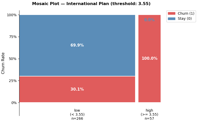
요금이 3.549 이상인 고객 수 : 57
요금이 3.549 이상인 고객 이탈율 : 1.0
# 모자이크 플롯
import matplotlib.pyplot as plt
from matplotlib.patches import Rectangle, Patch
groups = {
f'low\n(< {threshold:.2f})': low,
f'high\n(>= {threshold:.2f})': high,
}
total_n = len(df_yes)
gap = 0.02
fig, ax = plt.subplots(figsize=(8, 5))
x_cursor = 0
for label, series in groups.items():
n = len(series)
churn_rate = series.mean()
width = (n / total_n) - gap
ax.add_patch(Rectangle((x_cursor, 0), width, churn_rate,
color='#E05C5C', ec='white', lw=1.5))
ax.add_patch(Rectangle((x_cursor, churn_rate), width, 1 - churn_rate,
color='#5B8DB8', ec='white', lw=1.5))
if churn_rate > 0.05:
ax.text(x_cursor + width/2, churn_rate/2,
f'{churn_rate:.1%}', ha='center', va='center',
color='white', fontweight='bold', fontsize=11)
else:
ax.text(x_cursor + width/2, churn_rate + 0.04,
f'{churn_rate:.1%}', ha='center', va='bottom',
color='#E05C5C', fontweight='bold', fontsize=11)
if (1 - churn_rate) > 0.05:
ax.text(x_cursor + width/2, churn_rate + (1 - churn_rate)/2,
f'{1-churn_rate:.1%}', ha='center', va='center',
color='white', fontweight='bold', fontsize=11)
else:
ax.text(x_cursor + width/2, churn_rate - 0.04,
f'{1-churn_rate:.1%}', ha='center', va='top',
color='#5B8DB8', fontweight='bold', fontsize=11)
ax.text(x_cursor + width/2, -0.07,
f'{label}\nn={n}', ha='center', va='top', fontsize=10)
x_cursor += width + gap
ax.set_xlim(0, 1)
ax.set_ylim(-0.15, 1.05)
ax.set_xticks([])
ax.set_yticks([0, 0.25, 0.5, 0.75, 1.0])
ax.set_yticklabels(['0%', '25%', '50%', '75%', '100%'])
ax.set_ylabel('Churn Rate', fontsize=11)
ax.set_title(f'Mosaic Plot — International Plan (threshold: {threshold:.2f})',
fontsize=12, fontweight='bold', pad=15)
legend = [Patch(color='#E05C5C', label='Churn (1)'),
Patch(color='#5B8DB8', label='Stay (0)')]
ax.legend(handles=legend, fontsize=10,
bbox_to_anchor=(1.02, 1.0), loc='upper left', borderaxespad=0)
ax.spines[['top', 'right', 'bottom']].set_visible(False)
plt.tight_layout()
plt.show()
'아이티윌_데이터 분석 55기 > 강의내용 필기_분석(Python)' 카테고리의 다른 글
| #8 클래스 불균등 처리 (0) | 2026.06.15 |
|---|---|
| #7 7일차_독립성 검정, 적합도 검정, 클래스 불균등 처리 (0) | 2026.06.11 |
| #5 5일차_데이터 분석 과정, 로지스틱 회귀, 교호작용 (0) | 2026.06.08 |
| #4 4일차_복사 / SVM·RF 실습 / 모델링 파이프 라인 구축 / 분류 모델 / knn (0) | 2026.06.05 |
| #3 3일차_SVL 실습, 독립변수 스케일링 + 연습문제 및 문제풀이 (0) | 2026.06.04 |