01 SVL 실습
-01 실습1
-02 결과 시각화 : 히트맵
-03 그리드 서치
-04 실습2 (cancer의 종양의 양성 / 악성 분류 (SVC))
02 독립변수 스케일링
-01 방법
-02 코드구현
-03 주의사항
-04 올바른 스케일링 / 잘못된 스케일링 비교
03 'telecom_churn.csv' 실습
-01 인코딩
-02 실습
01 SVL 실습
-01 실습1
[ 예제 - SVM을 사용한 iris 품종 최적 분류 ]
# step1) 데이터 로딩
from sklearn.datasets import load_iris
iris = load_iris()
X = iris['data']
y = iris['target']
# step2) 데이터 분리
from sklearn.model_selection import train_test_split
train_x, test_x, train_y, test_y = train_test_split(X, y, random_state = 0)
# step3) 모델링
from sklearn.svm import SVC
m_svm = SVC()
m_svm.fit(train_x, train_y)
# step4) 평가
m_svm.score(train_x, train_y)
m_svm.score(test_x, test_y)
m_svm.score(train_x, train_y)
Out[16]: 0.9642857142857143

m_svm.score(test_x, test_y)
Out[17]: 0.9736842105263158
# step5) 매개변수 튜닝 (C, gamma 동시 튜닝)
C = [0.001, 0.01, 0.1, 1, 10, 100, 1000]
gamma = [0.001, 0.01, 0.1, 1, 10, 100, 1000]
score_tr = []; score_te = []
v_i = []; v_j = []
* 그리드 서치는 매개변수의 최적조합을 찾아준다.
for i in C :
for j in gamma :
m_svm = SVC(C = i, gamma = j)
m_svm.fit(train_x, train_y)
score_tr.append(m_svm.score(train_x, train_y))
score_te.append(m_svm.score(test_x, test_y))
v_i.append(i)
v_j.append(j)
import pandas as pd
df_result = pd.DataFrame({'C':v_i, 'gamma':v_j, 'train_score':score_tr, 'test_score':score_te})
pd.DataFrame({'C':v_i, 'gamma':v_j, 'train_score':score_tr, 'test_score':score_te})
Out[29]:
           C     gamma  train_score  test_score
0      0.001     0.001     0.366071    0.236842
1      0.001     0.010     0.366071    0.236842
2      0.001     0.100     0.366071    0.236842
3      0.001     1.000     0.366071    0.236842
4      0.001    10.000     0.366071    0.236842
5      0.001   100.000     0.366071    0.236842
6      0.001  1000.000     0.366071    0.236842
7      0.010     0.001     0.366071    0.236842
8      0.010     0.010     0.366071    0.236842
9      0.010     0.100     0.366071    0.236842
10     0.010     1.000     0.366071    0.236842
11     0.010    10.000     0.366071    0.236842
12     0.010   100.000     0.366071    0.236842
13     0.010  1000.000     0.366071    0.236842
14     0.100     0.001     0.366071    0.236842
15     0.100     0.010     0.696429    0.578947
16     0.100     0.100     0.937500    0.921053
17     0.100     1.000     0.955357    0.973684
18     0.100    10.000     0.455357    0.289474
19     0.100   100.000     0.366071    0.236842
20     0.100  1000.000     0.366071    0.236842
21     1.000     0.001     0.696429    0.578947
22     1.000     0.010     0.937500    0.921053
23     1.000     0.100     0.973214    0.973684
24     1.000     1.000     0.973214    0.973684
25     1.000    10.000     1.000000    0.921053
26     1.000   100.000     1.000000    0.342105
27     1.000  1000.000     1.000000    0.236842
28    10.000     0.001     0.937500    0.921053
29    10.000     0.010     0.973214    0.973684
30    10.000     0.100     0.991071    0.973684
31    10.000     1.000     0.991071    0.973684
32    10.000    10.000     1.000000    0.921053
33    10.000   100.000     1.000000    0.447368
34    10.000  1000.000     1.000000    0.236842
35   100.000     0.001     0.973214    0.973684
36   100.000     0.010     0.982143    0.973684
37   100.000     0.100     0.982143    0.947368
38   100.000     1.000     1.000000    0.973684
39   100.000    10.000     1.000000    0.921053
40   100.000   100.000     1.000000    0.447368
41   100.000  1000.000     1.000000    0.236842
42  1000.000     0.001     0.982143    0.973684
43  1000.000     0.010     0.982143    0.947368
44  1000.000     0.100     0.991071    0.973684
45  1000.000     1.000     1.000000    0.973684
46  1000.000    10.000     1.000000    0.921053
47  1000.000   100.000     1.000000    0.447368
48  1000.000  1000.000     1.000000    0.236842
-02 결과 시각화 : 히트맵
import seaborn as sns
import matplotlib.pyplot as plt
fig, ax = plt.subplots(1,2)
array_tr = df_result['train_score'].values.reshape(len(C), len(gamma))
array_te = df_result['test_score'].values.reshape(len(C), len(gamma))
sns.heatmap(array_tr, xticklabels = gamma, yticklabels = C, annot = True, fmt = '.3f',
cmap = 'YlOrRd', linewidths = 0.5, ax = ax[0])
ax[0].set_title('SVM Train score heatmap')
ax[0].set_xlabel('gamma')
ax[0].set_ylabel('C')
sns.heatmap(array_te, xticklabels = gamma, yticklabels = C, annot = True, fmt = '.3f',
cmap = 'YlOrRd', linewidths = 0.5, ax = ax[1])
ax[1].set_title('SVM Test score heatmap')
ax[1].set_xlabel('gamma')
ax[1].set_ylabel('C')
plt.tight_layout()
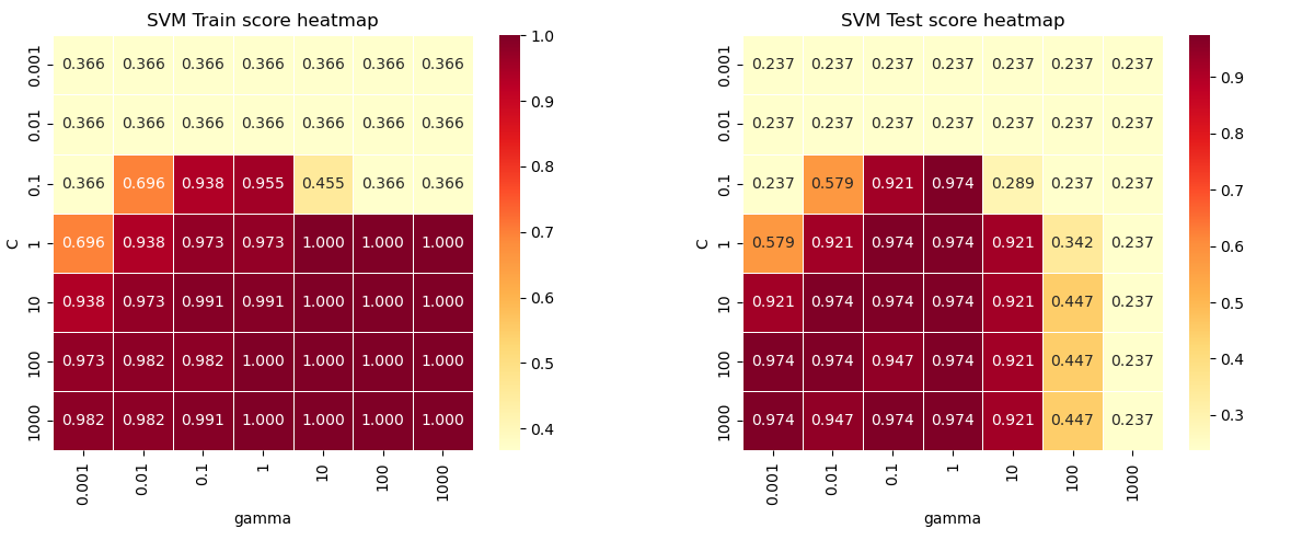
-03 그리드 서치
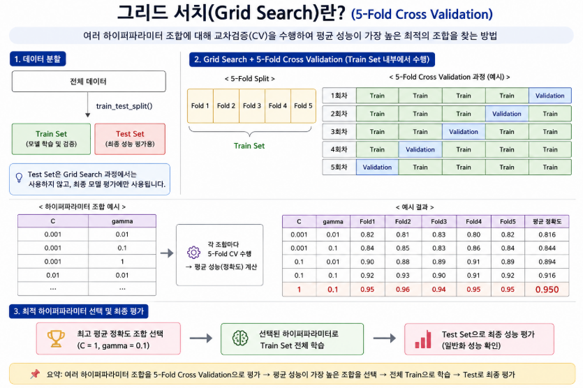
다양한 하이퍼파라미터 조합에 대해 교차검증을 수행하여 평균 성능이 가장 우수한 최적의 매개변수 조합을 탐색하는 기법이다.
from sklearn.model_selection import GridSearchCV
params = {'C' : [0.001, 0.01, 0.1, 1, 10, 100, 1000],
'gamma' : [0.001, 0.01, 0.1, 1, 10, 100, 1000]}
GridSearchCV(SVC(), params, cv = 5, scoring = 'accuracy')
▲ 정확도 (accuracy)라는 평가지표를 척도로 지정하였음
# ** 여러가지 scoring (평가척도) 값 확인
from sklearn.metrics import get_scorer_names
sorted(get_scorer_names())
sorted(get_scorer_names())
Out[54]:
['accuracy',
 'adjusted_mutual_info_score',
 'adjusted_rand_score',
 'average_precision',
 'balanced_accuracy',
 'completeness_score',
 'd2_absolute_error_score',
 'explained_variance',
 'f1',
 'f1_macro',
 'f1_micro',
 'f1_samples',
 ...
gridcv = GridSearchCV(SVC(), params, cv = 5, scoring = 'accuracy', n_jobs = -1)
≫ iris 데이터는 적은 수의 데이터이기 때문에 n_jobs = -1 설정을 진행하여도 처리 속도가 빠른 편이었으나, 추후 보다 큰 데이터 사용 시 주의를 해야 함
gridcv.fit(X, y) # 전체 데이터의 20%을 가지고 매개변수 평가를 진행함 (별도의 검증용 데이터셋이 없음)
gridcv.fit(train_x, train_y) # 훈련 데이터의 20%을 가지고 매개변수 평가를 진행함 (별도의 검증용 데이터셋이 존재함)
# 결과 해석
gridcv.best_params_ # {'C' : 1, 'gamma' : 0.1}
gridcv.best_params_         # {'C' : 1, 'gamma' : 0.1}
Out[62]: {'C': 1, 'gamma': 0.1}
gridcv.best_score_
gridcv.best_score_
Out[63]: np.float64(0.9800000000000001)
# step6) 최종 모형 선택
m_svm = SVC(C = 1, gamma = 0.1)
m_svm
# step7) 예측
m_svm.predict(X) # 정상
m_svm.predict_proba(X) # 에러
m_svm = SVC (probability = True) # 파이썬 SVM 모델에서는 probability = Ture일때만 predict_proba 호출 가능!
m_svm.fit(X, y)
m_svm.predict_proba(X) # 정상
-04 예제2 (cancer의 종양의 양성 / 악성 분류 (SVC))
# step1) 데이터 로딩
df = pd.read_csv('cancer.csv')
df.drop(columns = 'id', inplace = True)
y = df['diagnosis']
X = df.drop(columns = 'diagnosis')
# step2) 데이터 분리
from sklearn.model_selection import train_test_split
train_x, test_x, train_y, test_y = train_test_split(X, y, random_state = 0)
# step3) 모델링
from sklearn.svm import SVC
m_svm = SVC()
m_svm.fit(train_x, train_y)
# step4) 평가
m_svm.score(train_x, train_y)
m_svm.score(test_x, test_y)
m_svm.score(train_x, train_y)
Out[85]: 0.903755868544601

m_svm.score(test_x, test_y)
Out[86]: 0.9370629370629371
# step5) 매개변수 튜닝 (C, gamma 동시 튜닝)
C = [0.001, 0.01, 0.1, 1, 10, 100, 1000]
gamma = [0.001, 0.01, 0.1, 1, 10, 100, 1000]
score_tr = []; score_te = []
v_i = []; v_j = []
for i in C :
for j in gamma :
m_svm = SVC(C = i, gamma = j)
m_svm.fit(train_x, train_y)
score_tr.append(m_svm.score(train_x, train_y))
score_te.append(m_svm.score(test_x, test_y))
v_i.append(i)
v_j.append(j)
import pandas as pd
df_result = pd.DataFrame({'C':v_i, 'gamma':v_j, 'train_score':score_tr, 'test_score':score_te})
# ** 결과 시각화 : 히트맵
import seaborn as sns
import matplotlib.pyplot as plt
fig, ax = plt.subplots(1,2)
array_tr = df_result['train_score'].values.reshape(len(C), len(gamma))
array_te = df_result['test_score'].values.reshape(len(C), len(gamma))
sns.heatmap(array_tr, xticklabels = gamma, yticklabels = C, annot = True, fmt = '.3f',
cmap = 'YlOrRd', linewidths = 0.5, ax = ax[0])
ax[0].set_title('SVM Train score heatmap')
ax[0].set_xlabel('gamma')
ax[0].set_ylabel('C')
sns.heatmap(array_te, xticklabels = gamma, yticklabels = C, annot = True, fmt = '.3f',
cmap = 'YlOrRd', linewidths = 0.5, ax = ax[1])
ax[1].set_title('SVM Test score heatmap')
ax[1].set_xlabel('gamma')
ax[1].set_ylabel('C')
plt.tight_layout()

# ** 그리드 서치
from sklearn.model_selection import GridSearchCV
params = {'C' : [0.001, 0.01, 0.1, 1, 10, 100, 1000],
'gamma' : [0.001, 0.01, 0.1, 1, 10, 100, 1000]}
gridcv = GridSearchCV(SVC(), params, cv = 5, scoring = 'accuracy', n_jobs = -1)
gridcv.fit(X, y)
# 결과 해석
gridcv.best_params_ # {'C' : 1, 'gamma' : 0.1}
gridcv.best_score_
gridcv.best_params_         # {'C' : 1, 'gamma' : 0.1}
Out[114]: {'C': 1, 'gamma': 0.001}

gridcv.best_score_
Out[115]: np.float64(0.9226207110697097)
# step6) 최종 모형 선택
m_svm = SVC(C = 1, gamma = 0.001)
m_svm
02 독립변수 스케일링
변수가 갖는 범위에 민감한 모델 -> 거리기반 모델 (kmeans, knn 등), 회귀계수 비교 시, SVM, 신경망 모델 등
-01 방법
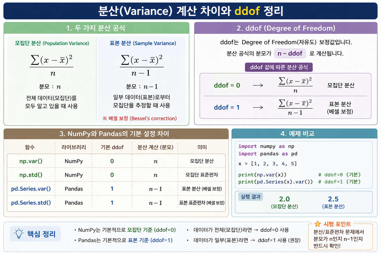
1) 표준화 (Standard scaling)
공식 : (X - X.mean()) / X.std()
표준화 이후의 평균을 0, 표준편차를 1로 맞추는 작업
음의 값을 가질 수 있음
2) 정규화 (Minmax scaling)
공식 : (X - X.min()) / (X.max() - X.min())
값들 중 최소를 0으로, 최대를 1로 맞추는 작업
3) Robust scaling
공식 : (X - q2) / (q3 - q1)
사분위수를 사용한 스케일링
-02 코드구현
[ 예제 - iris 스케일링 ]
1) 데이터 로딩
from sklearn.datasets import load_iris
iris = load_iris()
X = iris['data']
y = iris['target']
2) 직접 스케일링
(1) 표준화
(X - X.mean()) / X.std(axis = 0, ddof =1)
(X - X.mean()) / X.std(axis = 0, ddof =1)
Out[124]:
array([[ 1.97508381,  0.081447  , -1.16949078, -4.28278493],
       [ 1.7335572 , -1.06569381, -1.16949078, -4.28278493],
       [ 1.4920306 , -0.60683748, -1.22613843, -4.28278493],
       ...
(2) 정규화
(X - X.min(axis=0)) / (X.max(axis = 0) - X.min(axis = 0))
(X - X.min(axis=0)) / (X.max(axis = 0) - X.min(axis = 0))
Out[125]:
array([[0.22222222, 0.625     , 0.06779661, 0.04166667],
       [0.16666667, 0.41666667, 0.06779661, 0.04166667],
       [0.11111111, 0.5       , 0.05084746, 0.04166667],
       ...
(3) sklearn 함수로 스케일링
from sklearn.preprocessing import MinMaxScaler, RobustScaler, StandardScaler
import sklearn.preprocessing
dir(sklearn.preprocessing)
① 표준화
m_sc1 = StandardScaler()
m_sc1.fit(X) # 평균, 표준편차 계산
m_sc1.transform(X) # 수식대로 변수 변환
m_sc1.transform(X)  # 수식대로
Out[135]:
array([[-9.00681170e-01,  1.01900435e+00, -1.34022653e+00,
        -1.31544430e+00],
       [-1.14301691e+00, -1.31979479e-01, -1.34022653e+00,
        -1.31544430e+00],
       [-1.38535265e+00,  3.28414053e-01, -1.39706395e+00,
        -1.31544430e+00],
        ...
② 정규화
m_sc2 = MinMaxScaler()
m_sc2.fit(X) # 평균, 표준편차 계산
m_sc2.transform(X) # 수식대로 변수 변환
m_sc2.transform(X)  # 수식대로 변수 변환
Out[138]:
array([[0.22222222, 0.625     , 0.06779661, 0.04166667],
       [0.16666667, 0.41666667, 0.06779661, 0.04166667],
       [0.11111111, 0.5       , 0.05084746, 0.04166667],
       ...
③ Robust scaler
m_sc3 = RobustScaler()
m_sc3.fit_transform(X)
m_sc3.fit_transform(X)
Out[141]:
array([[-0.53846154,  1.        , -0.84285714, -0.73333333],
       [-0.69230769,  0.        , -0.84285714, -0.73333333],
       [-0.84615385,  0.4       , -0.87142857, -0.73333333],
       ...
-03 주의사항
train_x, test_x 분리된 경우 스케일링 시
1) 각각 fit 진행 (권고 x)
- train / test의 변환 기준이 달라짐
- 원래 데이터의 성격이 왜곡됨
(본래 데이터의 상대적인 위치가 왜곡)
train_x 에 대해 fit_transform
test_x 에 대해 fit_transform
m_sc1 = StandardScaler()
m_sc1.fit_transform(train_x)
m_sc1.fit_transform(test_x)
2) train에 대해서만 fit 진행
- train / test의 변환 성격이 유지됨
- 왜곡 x
m_sc1 = StandardScaler()
m_sc1.fit_transform(train_x)
m_sc1.fit_transform(test_x)
fit를 한 번만 수행해야 한다.
-04 올바른 스케일링 / 잘못된 스케일링 비교
iris 데이터의 두 설명변수를 각각 x축, y축으로 가지는 산점도를 그리고 올바른 스케일링 결과와 잘못된 스케일링 결과를 제시
두 설명변수(X1, X2)를 각각 x축, y축으로 가지는 산점도를 그려서 원본과 일치하는 스케일링 결과 확인
# 1) 데이터 로딩
from sklearn.datasets import load_iris
iris = load_iris()
X = iris['data']
y = iris['target']
# 2) 데이터 분리
from sklearn.model_selection import train_test_split
train_x, test_x, train_y, test_y = train_test_split(X, y, random_state=0)
# ▲ 원본을 가지고 있으면 분리 전에 (하나의 집합일 때) 스케일링을 진행하면 된다.
# 공모전, 기사 시험의 경우 데이터가 아예 나누어져서 제공되기 때문에 각각 스케일링을 진행한다.
# 3) 스케일링 진행
from sklearn.preprocessing import MinMaxScaler
# 1) 올바른 스케일링
m_sc1 = MinMaxScaler()
train_x_sc1 = m_sc1.fit_transform(train_x)
test_x_sc1 = m_sc1.transform(test_x)
# 2) 잘못된 스케일링
m_sc2 = MinMaxScaler()
train_x_sc2 = m_sc2.fit_transform(train_x)
m_sc3 = MinMaxScaler()
test_x_sc2 = m_sc3.fit_transform(test_x)
# 4) 시각화
import matplotlib.pyplot as plt
fig, ax = plt.subplots(1,3)
ax[0].scatter(train_x[:,0], train_x[:,1], c = 'b', label='train')
ax[0].scatter(test_x[:,0], test_x[:,1], c = 'r', label='test')
ax[0].legend()
ax[0].set_title('scatter')
ax[1].scatter(train_x_sc1[:,0], train_x_sc1[:,1], c = 'b', label='train')
ax[1].scatter(test_x_sc1[:,0], test_x_sc1[:,1], c = 'r', label='test')
ax[1].legend()
ax[1].set_title('true scatter')
ax[2].scatter(train_x_sc2[:,0], train_x_sc2[:,1], c = 'b', label='train')
ax[2].scatter(test_x_sc2[:,0], test_x_sc2[:,1], c = 'r', label='test')
ax[2].legend()
ax[2].set_title('false scatter')

[ SVM 모델의 스케일링 전/후 비교(cancer data) ]
# STEP1) 데이터 로딩
cancer = pd.read_csv('cancer.csv')
cancer.drop(columns = 'id', inplace = True)
y = cancer['diagnosis']
X = cancer.drop(columns = 'diagnosis')
# STEP2) 스케일링
from sklearn.preprocessing import StandardScaler
m_sc = StandardScaler()
X_sc = m_sc.fit_transform(X)
# STEP3) 데이터 분리
from sklearn.model_selection import train_test_split
train_x, test_x, train_x_sc, test_x_sc, train_y, test_y = train_test_split(X, X_sc, y, random_state=0)
# STEP4) 모델링
from sklearn.svm import SVC
m_svm1 = SVC()
m_svm1.fit(train_x, train_y)
m_svm2 = SVC()
m_svm2.fit(train_x_sc, train_y)
# STEP5) 평가
m_svm1.score(train_x, train_y) # 0.9037
m_svm1.score(test_x, test_y) # 0.9370
m_svm2.score(train_x_sc, train_y) # 0.9859
m_svm2.score(test_x_sc, test_y) # 0.9650
# STEP6) 매개변수 튜닝
from sklearn.model_selection import GridSearchCV
params = {'C':[0.001, 0.01, 0.1, 1, 10, 100, 1000],
'gamma':[0.001, 0.01, 0.1, 1, 10, 100, 1000]}
gridcv = GridSearchCV(SVC(), params, cv=5, scoring='accuracy', n_jobs=-1)
gridcv.fit(train_x_sc, train_y)
# 결과 해석
gridcv.best_params_ # {'C': 10, 'gamma': 0.01}
gridcv.best_score_ # 0.9858
gridcv.score(train_x_sc, train_y) # 0.9859
gridcv.score(test_x_sc, test_y) # 0.9790
03 'telecom_churn.csv' 실습
SVM 모델의 경우 one hot encoding이 맞다.
그러나 해당 데이터의 경우 당분간은 label encoding으로 진행한다.
-01 인코딩
문자 데이터 -> 숫자 변환
1) 라벨인코딩
s1 = pd.Series(['A','A','B','C','C','C'])
(1) 직접 변환
map_rule = {'A':0, 'B':1, 'C':2}
s1.map(map_rule)
(2) 인코딩 함수
df['state'].unique()
df['state'].unique()
Out[197]:
array(['KS', 'OH', 'NJ', 'OK', 'AL', 'MA', 'MO', 'LA', 'WV', 'IN', 'RI',
       'IA', 'MT', 'NY', 'ID', 'VT', 'VA', 'TX', 'FL', 'CO', 'AZ', 'SC',
       'NE', 'WY', 'HI', 'IL', 'NH', 'GA', 'AK', 'MD', 'AR', 'WI', 'OR',
       'MI', 'DE', 'UT', 'CA', 'MN', 'SD', 'NC', 'WA', 'NM', 'NV', 'DC',
       'KY', 'ME', 'MS', 'TN', 'PA', 'CT', 'ND'], dtype=object)
m_ec.fit_transform(df['state'])
m_ec.fit_transform(df['state'])
Out[204]: array([16, 35, 31, ..., 39,  6, 42], shape=(3333,))
2) 원핫인코딩
pd.get_dummies?
Signature:
pd.get_dummies(
    data,
    prefix=None,
    prefix_sep: 'str | Iterable[str] | dict[str, str]' = '_',
    dummy_na: 'bool' = False,
    columns=None,
    sparse: 'bool' = False,
    drop_first: 'bool' = False,
    dtype: 'NpDtype | None' = None,
) -> 'DataFrame'
Docstring:
Convert categorical variable into dummy/indicator variables.
pd.get_dummies(df['state']).astype('int')
pd.get_dummies(df['state']).astype('int')
Out[207]:
      AK  AL  AR  AZ  CA  CO  CT  DC  DE  ...  TN  TX  UT  VA  VT  WA  WI  WV  WY
0      0   0   0   0   0   0   0   0   0  ...   0   0   0   0   0   0   0   0   0
1      0   0   0   0   0   0   0   0   0  ...   0   0   0   0   0   0   0   0   0
2      0   0   0   0   0   0   0   0   0  ...   0   0   0   0   0   0   0   0   0
3      0   0   0   0   0   0   0   0   0  ...   0   0   0   0   0   0   0   0   0
4      0   0   0   0   0   0   0   0   0  ...   0   0   0   0   0   0   0   0   0
  ..  ..  ..  ..  ..  ..  ..  ..  ..  ...  ..  ..  ..  ..  ..  ..  ..  ..  ..
3328   0   0   0   1   0   0   0   0   0  ...   0   0   0   0   0   0   0   0   0
3329   0   0   0   0   0   0   0   0   0  ...   0   0   0   0   0   0   0   1   0
3330   0   0   0   0   0   0   0   0   0  ...   0   0   0   0   0   0   0   0   0
3331   0   0   0   0   0   0   1   0   0  ...   0   0   0   0   0   0   0   0   0
3332   0   0   0   0   0   0   0   0   0  ...   1   0   0   0   0   0   0   0   0

[3333 rows x 51 columns
-02 실습
# 1. 데이터 로딩 및 설명
pd.set_option('display.max_column', None)
df = pd.read_csv('telecom_churn.csv')
# X, y 분리
X = df.drop(columns='churn')
y = df['churn']
# 데이터 설명
df.info()
# Column Non-Null Count Dtype
# --- ------ -------------- -----
# 0 state 3333 non-null object 미국 주(State) 코드 (KS, OH, NJ 등)
# 1 account length 3333 non-null int64 계정 사용 기간 (일 수)
# 2 area code 3333 non-null int64 지역 전화 코드 (408 / 415 / 510)
# 3 phone number 3333 non-null object 전화번호
# 4 international plan 3333 non-null object 국제전화 요금제 가입 여부 (yes/no)
# 5 voice mail plan 3333 non-null object 음성 사서함 요금제 가입 여부 (yes/no)
# 6 number vmail messages 3333 non-null int64 음성 사서함 메시지 수
# 7 total day minutes 3333 non-null float64 낮 시간대 총 통화 시간 (분)
# 8 total day calls 3333 non-null int64 낮 시간대 총 통화 횟수
# 9 total day charge 3333 non-null float64 낮 시간대 총 요금
# 10 total eve minutes 3333 non-null float64 저녁 시간대 총 통화 시간 (분)
# 11 total eve calls 3333 non-null int64 저녁 시간대 총 통화 횟수
# 12 total eve charge 3333 non-null float64 저녁 시간대 총 요금
# 13 total night minutes 3333 non-null float64 야간 시간대 총 통화 시간 (분)
# 14 total night calls 3333 non-null int64 야간 시간대 총 통화 횟수
# 15 total night charge 3333 non-null float64 야간 시간대 총 요금
# 16 total intl minutes 3333 non-null float64 국제전화 총 통화 시간 (분)
# 17 total intl calls 3333 non-null int64 국제전화 총 통화 횟수
# 18 total intl charge 3333 non-null float64 국제전화 총 요금
# 19 customer service calls 3333 non-null int64 고객센터 전화 횟수
# 20 churn 3333 non-null bool 타겟 — 고객 이탈 여부 (True/False)
독립성 검정 object type 지우기로했음
전화번호 지우기로 했음
# 2. 라벨 인코딩
obj_cols = X.select_dtypes(include='object').columns # 문자형 컬럼만 선택
num_cols = X.select_dtypes(exclude='object').columns # 숫자형 컬럼만 선택
from sklearn.preprocessing import LabelEncoder
for colname in obj_cols:
m_ec = LabelEncoder()
X[colname] = m_ec.fit_transform(X[colname]) # X에서 문자형 컬럼을 라벨인코딩 변환 후 바로 덮어쓰기
# 3. 스케일링
from sklearn.preprocessing import MinMaxScaler
X_sc = X.copy() # X와 동일한 X_sc copy 데이터 생성
for colname in num_cols:
m_sc = MinMaxScaler()
X_sc[colname] = m_sc.fit_transform(X_sc[[colname]]) # X_sc에서 수치형 컬럼만 선택(2차원으로)하여 스케일링 변환 후 바로 덮어쓰기
# ** 데이터 설명
# X : 문자 데이터 라벨인코딩 완료, 숫자 데이터 스케일링 진행 안함
# X_sc : 문자 데이터 라벨인코딩 완료, 숫자 데이터 스케일링 진행 함
'아이티윌_데이터 분석 55기 > 강의내용 필기_분석(Python)' 카테고리의 다른 글
| #6 교호작용 및 효과 검증 (0) | 2026.06.09 |
|---|---|
| #5 5일차_데이터 분석 과정, 로지스틱 회귀, 교호작용 (0) | 2026.06.08 |
| #4 4일차_복사 / SVM·RF 실습 / 모델링 파이프 라인 구축 / 분류 모델 / knn (0) | 2026.06.05 |
| #2 2일차_랜덤포레스트 (분류), SVM (Support Vector Machine) (0) | 2026.06.02 |
| #1 1일차_ 분석 프로세스, 머신러닝 기반 모델링 기법, 의사결정나무 (0) | 2026.06.01 |