01 랜덤포레스트 (분류)
-01 트리의 성장
-02 랜덤포레스트의 장단점
-03 분석코드
02 SVM (Support Vector Machine)
01 랜덤포레스트 (분류)
- 앙상블 모형 : 동일하거나 다른 모델을 결합하여 하나의 의사결정을 하도록 만드는 과정이다.
- 여러 개의 의사결정나무를 결합한 앙상블 모형이다.
- 목적은 서로 다른 트리를 구성함으로써 :
1) 부트스트랩 : 복원추출을 허용하여 크기는 같지만 구성이 다른 샘플을 만드는 과정
2) 임의성정도 (max_features) : 가지 성장 시 (split) 일부 독립변수만 고려하여 자식노드로 분할
3) 배깅 (bootstrap + aggregating) : 각 트리의 학습 결과를 최종 결합 (다수결, 평균)하여 하나의 결과를 만드는 과정
-01 트리의 성장
1) 불순도 감소량이 가장 큰 변수를 사용하여 분할을 진행함 (분류트리)
> 불순도 : gini index, entropy...
> 불순도 감소량 : 정보이득 (IG : Information Gain), 카이제곱통계량 (적합도 검정 : 멘델의 유전법칙을 기억하기)
2) 분산 감소량이 가장 큰 변수를 사용하여 분할을 진행함 (회귀트리)
-02 랜덤포레스트의 장단점
1) 장점
- 스케일에 민감하지 않다.
- 이상치에 민감하지 않다.
- 변수 중요도를 계산 · 제공하므로 변수 선택에 대한 부담이 적다.
2) 단점
- 트리가 많을수록 학습 속도과 느려진다.
(병렬처리 → CPU core 수가 많을수록 병렬처리의 효과가 극대화된다.)
-03 분석코드
import sklearn.ensemble
dir(sklearn.ensemble)
* RF 기반의 이상치 검정 시 : IsolationForest
import sklearn.ensemble import RandomForestClassifier
RandomForestClassifier(n_estimators = 100,
...,
max_features = 'sqrt',
n_jobs, # 병렬처리할 CPU processor 수
class_weight =, # balanced (클래스 불균등 시 가중치 조절 방식)
) # {0:1, 1:5} 직접 클래스별 가중치 전달 가능
# n_jobs = -1로 설정(모든 프로세스를 다 사용) 시 다른 업무가 비정상종료 될 수 있다.
[ 예제 - iris data 종 분류 (RF) ]
# step1) 데이터 불러오기
import pandas as pd
iris = pd.read_csv('iris.csv', header = None)
iris
Out[7]:
       0    1    2    3               4
0    5.1  3.5  1.4  0.2     Iris-setosa
1    4.9  3.0  1.4  0.2     Iris-setosa
2    4.7  3.2  1.3  0.2     Iris-setosa
3    4.6  3.1  1.5  0.2     Iris-setosa
4    5.0  3.6  1.4  0.2     Iris-setosa
..   ...  ...  ...  ...             ...
145  6.7  3.0  5.2  2.3  Iris-virginica
146  6.3  2.5  5.0  1.9  Iris-virginica
147  6.5  3.0  5.2  2.0  Iris-virginica
148  6.2  3.4  5.4  2.3  Iris-virginica
149  5.9  3.0  5.1  1.8  Iris-virginica

[150 rows x 5 columns]
iris.columns = ['sepal.length','sepal.width','petal.length','petal.width','species']
iris['species'] = iris['species'].str.replace('Iris-','')
y = iris['species']
X = iris.drop(columns = 'species')
* y의 경우 라벨 인코딩, 딥러닝 사용 시 원핫인코딩
# step2) 데이터 분리
from sklearn.model_selection import train_test_split
train_x, test_x, train_y, test_y = train_test_split(X, y, random_state = 0)
# step3) 모델링
from sklearn.ensemble import RandomForestClassifier
m_rf = RandomForestClassifier()
m_rf.fit(train_x, train_y)
# step4) 평가
m_rf.score(train_x, train_y)
m_rf.score(train_x, train_y)
Out[19]: 1.0
m_rf.score(test_x, test_y)
m_rf.score(test_x, test_y)
Out[20]: 0.9736842105263158
# step5) 매개변수 튜닝
1) max_features
설명변수의 후보이기 때문에 최솟값은 1, 최댓값은 설명변수의 갯수만큼 설정이 가능하다.
score_tr = []; score_te = []
for i in range(1,5) :
m_rf = RandomForestClassifier(random_state = 0, max_features = i)
m_rf.fit(train_x, train_y)
score_tr.append(m_rf.score(train_x, train_y))
score_te.append(m_rf.score(test_x, test_y))
import matplotlib.pyplot as plt
plt.plot(range(1,5), score_tr, label = 'train_score')
plt.plot(range(1,5), score_te, label = 'train_score')
plt.xthicks(range(1,5))
plt.legend()
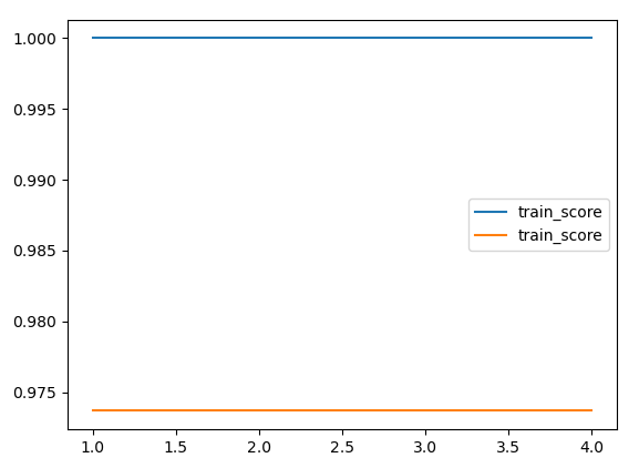
max_features는 RandomForest의 하이퍼파라미터로, Iris 데이터의 설명변수 개수(feature 수)가 4개뿐이라서 max_features를 1~4로 바꿔도 큰 차이가 나지 않는다.
# 2) min_sample_split
score_tr = []; score_te = []
for i in range(2,11) :
m_rf = RandomForestClassifier(random_state = 0, min_samples_split = i)
m_rf.fit(train_x, train_y)
score_tr.append(m_rf.score(train_x, train_y))
score_te.append(m_rf.score(test_x, test_y))
import matplotlib.pyplot as plt
plt.plot(range(2,11), score_tr, label = 'train_score')
plt.plot(range(2,11), score_te, label = 'train_score')
plt.xthicks(range(2,11))
plt.ylim([0.96, 1.01])
plt.legend()
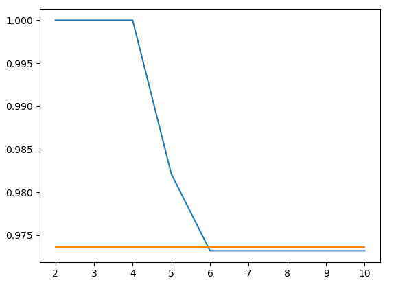
5 정도가 적합하며 6부터는 과소적합 (트리의 depth가 지나치게 짧음) 으로 판단된다.
# step6) 최종모형 선택
- 매개변수 튜닝값으로 학습
- 전체 학습
m_rf = RandomForestClassifier(random_state = 0, max_features= 5)
m_rf.fit(X,y)
# step7) 예측
m_rf.predict(X)
m_rf.predict(X)
Out[39]:
array(['setosa', 'setosa', 'setosa', 'setosa', 'setosa', 'setosa',
       'setosa', 'setosa', 'setosa', 'setosa', 'setosa', 'setosa',
       'setosa', 'setosa', 'setosa', 'setosa', 'setosa', 'setosa',
m_rf.predict_proba(X)
m_rf.predict_proba(X)
Out[40]:
array([[1.  , 0.  , 0.  ],
       [1.  , 0.  , 0.  ],
       [1.  , 0.  , 0.  ],
       [1.  , 0.  , 0.  ],
[ 예제 - cancer 데이터에 대한 종양의 양성 / 악성 여부 예측 (RF) ]
# step1) 데이터 로딩
df = pd.read_csv('cancer.csv')
df.drop(columns = 'id', inplace = True)
y = df['diagnosis']
X = df.drop(columns = 'diagnosis')
# step2) 데이터 분리
from sklearn.model_selection import train_test_split
train_x, test_x, train_y, test_y = train_test_split(X,y,random_state = 0)
# step3) 모델링
from sklearn.ensemble import RandomForestClassifier
m_rf = RandomForestClassifier()
m_rf.fit(train_x, train_y)
# ** 결과 확인
cancer_imp = pd.Series(m_rf.feature_importances_, index = X.columns)
cancer_imp.sort_values(ascending = False)
cancer_imp.sort_values(ascending = False)
Out[72]:
perimeter_worst            0.162153
concave_points_worst       0.134474
radius_worst               0.130529
area_worst                 0.097703
concave_points_mean        0.093264
concavity_mean             0.055360
area_mean                  0.050653
perimeter_mean             0.048600
area_se                    0.031843
concavity_worst            0.026910
radius_mean                0.025477
texture_worst              0.021847
compactness_worst          0.016408
perimeter_se               0.012968
smoothness_worst           0.012051
texture_mean               0.010744
radius_se                  0.008812
smoothness_mean            0.007572
symmetry_worst             0.006919
compactness_se             0.005863
compactness_mean           0.005707
symmetry_mean              0.005283
texture_se                 0.004420
fractal_dimension_se       0.004148
smoothness_se              0.003874
fractal_dimension_worst    0.003801
fractal_dimension_mean     0.003579
symmetry_se                0.003112
concave_points_se          0.002971
concavity_se               0.002956
dtype: float64
변수 중요도의 경우 Decision Tree와 Random Forest 간에 일부 차이가 나타날 수밖에 없다.
그러나 변수 선택 결과는 래퍼(Wrapper), 필터(Filter), 임베디드(Embedded) 기법 등 적용하는 방법에 따라 달라질 수 있으므로, 하나의 결과를 맹신하는 것보다 다양한 기법을 비교·검토하는 과정이 필요하다.
또한 최종 변수 선정에는 분석가의 도메인 지식과 판단이 함께 반영되어야 한다.
# step5) 매개변수 튜닝
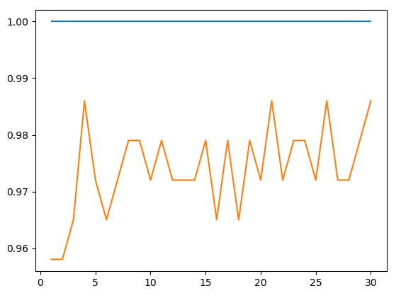
1) max_features
len(X.columns) # 30
score_tr = []; score_te = []
for i in range(1,31) :
m_rf = RandomForestClassifier(random_state = 0, max_features = i)
m_rf.fit(train_x, train_y)
score_tr.append(m_rf.score(train_x, train_y))
score_te.append(m_rf.score(test_x, test_y))
import matplotlib.pyplot as plt
plt.plot(range(1,31), score_tr, label = 'train_score')
plt.plot(range(1,31), score_te, label = 'train_score')
plt.xthicks(range(1,31))
plt.legend()
# 2) min_sample_split
score_tr = []; score_te = []
for i in range(2,21) :
m_rf = RandomForestClassifier(random_state = 0, min_samples_split = i)
m_rf.fit(train_x, train_y)
score_tr.append(m_rf.score(train_x, train_y))
score_te.append(m_rf.score(test_x, test_y))
import matplotlib.pyplot as plt
plt.plot(range(2,21), score_tr, label = 'train_score')
plt.plot(range(2,21), score_te, label = 'train_score')
plt.xthicks(range(2,21))
plt.ylim([0.96, 1.01])
plt.legend()

# step6) 최종모형 선택
m_rf = RandomForestClassifier(random_state = 0, min_samples_split= 6, max_features = 4)
m_rf.fit(X,y)
# step7) 예측
m_rf.predict_proba(X) # Benign, Malignant 순서대로 도출
m_rf.predict_proba(X)
Out[90]:
array([[0.0563254 , 0.9436746 ],
       [0.03281385, 0.96718615],
       [0.        , 1.        ],
       ...,
       [0.03408333, 0.96591667],
       [0.        , 1.        ],
       [0.988     , 0.012     ]], shape=(569, 2))
y.unique()
y.unique()
Out[91]: array(['Malignant', 'Benign'], dtype=object)
result = m_rf.predict_proba(X)[:,1]
result
Out[98]:
array([0.9436746 , 0.96718615, 1.        , 0.89759127, 0.93895238,
       0.88954365, 1.        , 0.9725    , 0.96122222, 0.95407143,
       0.79592063, 1.        , 0.9979798 , 0.85550794, 0.95963095,
       0.995     , 0.95783333, 1.        , 1.        , 0.00366667,
       0.023     , 0.        , 0.96966667, 0.99509091, 1.        ,
# step8) 결과 제출
df = pd.DataFrame({'pred':result})
df.to_csv('result.csv', index = False)
02 SVM (Support Vector Machine)
- 분류 / 회귀 가능
- 예측력이 강하고 쉽게 과적합 되지 않는 모델 (파라미터 조절 필요)
- 계산량이 많고 모델 내부가 복잡함 → 해석의 어려움 (예측 초점)
- 고차원 데이터, 많은 양의 데이터 학습에 유리x
* 용어 정리
1) 결정경계 : 클래스를 분류하는 경계
2) 초평면 : 다차원 공간에서의 분류경계
3) 커널트릭 : 실제 고차원 데이터로 변경하지는 않지만 마치 고차원 데이터로 변경하는 연산식(함수)을 통해 고차원 매핑을 유도하는 과정 (함수)
- kernel = 'rbf' default, 가장 많이 사용함, 비선형결정경계를 유도하는 차원 확장
- kernel = 'poly' 다항식 추가(x1**2, x1**3)
- kernel = 'sigmoid'
- kernel = 'linear'
4) 슬랙변수 : 결정경계를 만드는 과정에서 허용하는 오차, 슬랙변수의 강도를 C 매개변수로 결정
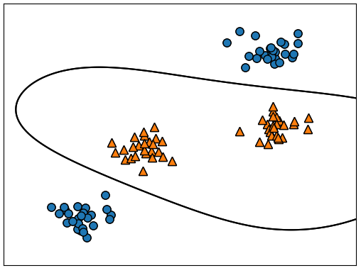
C 작으면 : 오차허용 O -> 모델 복잡도가 낮아짐 (선형 경계)
C 크면 : 오차허용 X -> 모델 복잡도가 증가함 (비선형 경계)
5) gamma : 결정경계를 구성하는 데이터포인트의 허용 범위를 결정하는 매개변수
gamma가 작을수록 -> 전체 데이터를 고려하여 결정경계 생성 -> 서포트벡터의 가중치가 상대적으로 작게 설정됨 -> 단순 경계
gamma가 커질수록 -> 결정경계 인근 데이터만 고려하여 결정경계 생성 -> 서포트벡터의 가중치가 상대적으로 높게 설정됨 -> 복잡한 경계
예) x1, x2로 2차원 공간선상에서 분류 경계 복잡
x2**2 추가 -> 3차원 공간선상에서 분류 경계 단순
f(x) -> 고차원 데이터
[ 예제 - SVM 모델의 결정경계 시각화 ]
# step1) 데이터 로딩
from sklearn.datasets import make_blobs
X, y = make_blobs(centers = 4, random_state = 8)
y = y % 2 # 이진클래스 분류과제를 위해 2로 나눈 나머지값으로 변경
# step2) 분포 시각화
# pip install mglearn
import mglearn
mglearn.discrete_scatter(X[:,0], # x축 좌표 (첫 번째 설명변수)
X[:,1], # y축 좌표 (두 번째 설명변수)
y=y, # class 정보 (target 변수)
s=8) # 점 크기
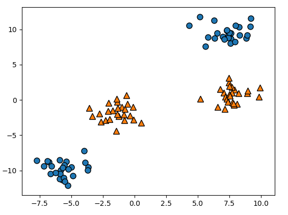
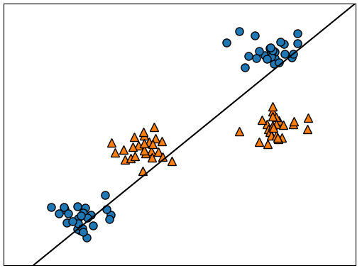
선형결정경계가 불가능한 상황이다.
# step3) 선형 분류기를 사용한 선형 결정 경계 생성
from sklearn.svm import LinearSVC, SVC
import sklearn.svm
dir(sklearn.svm)
m_svc1 = LinearSVC()
m_svc1.fit(X,y) # 결정경계를 생성하는 과정
** 결과 확인
m_svc1.coef_ # x1, x2에 대한 기울기
m_svc1.intercept_ # 절편
** 결정경계 시각화
mglearn.plots.plot_2d_separator(classifier, # 분류모델
X) # 설명변수 집합
mglearn.plots.plot_2d_separator(m_svc1, X)
# step4) 비선형 분류기를 사용한 선형 결정 경계 생성
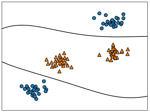
m_svc2 = SVC()
m_svc2.fit(X,y)
mglearn.discrete_scatter(X[:,0], X[:,1], y=y, s=8)
mglearn.plots.plot_2d_separator(m_svc2, X)
** C의 변화에 따른 결정경계 시각화
** C는 오차 허용 수준의 개념
m_svc3 = SVC(C = 0.001)
m_svc3.fit(X,y)
mglearn.discrete_scatter(X[:,0], X[:,1], y=y, s=8)
mglearn.plots.plot_2d_separator(m_svc3,X)
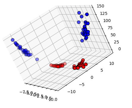
# step5) 차원 증가에 따른 결정경계(초평면) 시각화
import numpy as np
X_new = np.hstack([X, X[:,1:2]**2])
# ** 3차원 공간에 시각화
from mpl_toolkits.mplot3d import axes3d
fig = plt.figure()
ax = fig.add_subplot(111, projection='3d')
# y==0일때 산점도)
ax.scatter(X_new[y==0, 0], # X축 좌표
X_new[y==0, 1], # Y축 좌표
X_new[y==0, 2], # Z축 좌표
c = 'b', # 점 색
s=60, # 점 크기
edgecolors = 'k') # 점 테두리 색
# y==1일때 산점도)
ax.scatter(X_new[y==1, 0], # X축 좌표
X_new[y==1, 1], # Y축 좌표
X_new[y==1, 2], # Z축 좌표
c = 'r', # 점 색
s=60, # 점 크기
edgecolors = 'k') # 점 테두리 색
# 초평면(분류평면) 유도 및 시각화
m_svc4 = LinearSVC()
m_svc4.fit(X_new, y)
intercept = m_svc4.intercept_ # 초평면 절편
coef = m_svc4.coef_.ravel() # 초평면 기울기
# 시각화
np.linspace(-3,3,1000) # -3부터 3까지 1000개로 균등 분할
xx = np.linspace(X_new[:,0].min() - 2, X_new[:,0].max() + 2, 1000)
yy = np.linspace(X_new[:,1].min() - 2, X_new[:,1].max() + 2, 1000)
XX, YY = np.meshgrid(xx, yy) # 2차원 공간안의 좌표값으로 변환
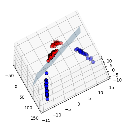
# ** f(x) = a1X + a2Y + a3Z + b 의 결정경계 수식으로부터 f(x)의 값이 양수일 경우 양의 클래스로,
# 음수을 경우 음의 클래스로 분류하게 된다.
# 따라서, 양과 음을 분류하기 위해 f(x)값이 0일때를 기준으로 Z좌표를 얻게되면
ZZ = (coef[0] * XX + coef[1] * YY + intercept) / -coef[2]
ax.plot_surface(XX, YY, ZZ, alpha = 0.3)
[ 예제 - SVM을 사용한 iris 데이터의 분류 경계 시각화 ]
# step1) 데이터 로딩
from sklearn.datasets import load_iris
iris = load_iris()
X = iris['data']
y = iris['target']
# ** 이진 클래스 분류 문제를 위한 데이터 선택
X = X[y != 0,:][:,[2,3]] # 3,4번째 설명변수만 선택하여 분석 시도
y = y[y != 0] # 첫번째 클래스를 제외한 나머지 클래스 선택
# step2) 분포 시각화
mglearn.discrete_scatter(X[:,0], X[:,1], y=y, s=8)
# step3) 선형 분류기를 사용한 선형 결정 경계 생성
from sklearn.svm import LinearSVC, SVC
import sklearn.svm
m_svc1 = LinearSVC()
m_svc1.fit(X,y) # 결정경계를 생성하는 과정
** 결과 확인
m_svc1.coef_ # x1, x2에 대한 기울기
m_svc1.intercept_ # 절편
** 결정경계 시각화
mglearn.plots.plot_2d_separator(classifier, # 분류모델
X) # 설명변수 집합
mglearn.plots.plot_2d_separator(m_svc1, X)

# step4) 비선형 분류기를 사용한 선형 결정 경계 생성
m_svc2 = SVC()
m_svc2.fit(X,y)
mglearn.discrete_scatter(X[:,0], X[:,1], y=y, s=8)
mglearn.plots.plot_2d_separator(m_svc2, X)
** C의 변화에 따른 결정경계 시각화
mglearn.plots.plot_2d_separator(m_svc2, X)
m_svc3 = SVC(C = 0.001)
m_svc3.fit(X,y)
mglearn.discrete_scatter(X[:,0], X[:,1], y=y, s=8)
mglearn.plots.plot_2d_separator(m_svc3,X)
m_svc3 = SVC(C = 0.01)
m_svc3.fit(X,y)
mglearn.discrete_scatter(X[:,0], X[:,1], y=y, s=8)
mglearn.plots.plot_2d_separator(m_svc3,X)
m_svc3 = SVC(C = 1)
m_svc3.fit(X,y)
mglearn.discrete_scatter(X[:,0], X[:,1], y=y, s=8)
mglearn.plots.plot_2d_separator(m_svc3,X)
** gamma의 변화에 따른 결정경계 시각화
m_svc3 = SVC(gamma = 0.1)
m_svc3.fit(X,y)
mglearn.discrete_scatter(X[:,0], X[:,1], y=y, s=8)
mglearn.plots.plot_2d_separator(m_svc3,X)
m_svc3 = SVC(gamma = 10)
m_svc3.fit(X,y)
mglearn.discrete_scatter(X[:,0], X[:,1], y=y, s=8)
mglearn.plots.plot_2d_separator(m_svc3,X)
m_svc3 = SVC(gamma = 100)
m_svc3.fit(X,y)
mglearn.discrete_scatter(X[:,0], X[:,1], y=y, s=8)
mglearn.plots.plot_2d_separator(m_svc3,X)
# 참고 : 분석기사실기 / 공모전 분석
X : train / test
y : train
- 데이터만 제공됨
- 성별 예측 (분류분석과제)
pd.read_csv('X_train.csv', encoding = 'cp949') # raw data(x)
pd.read_csv('X_test.csv', encoding = 'cp949') # raw data(y)
-> raw data를 사용하여 다시 75 : 25 로 데이터를 분할하여 학습용 데이터를 만들어야 한다.
-> 평가 결과를 토대로 최종 모형을 만들고 아래 제출용 데이터셋에 대한 예측 결과를 제출해야 한다.
pd.read_csv('y_train.csv', encoding = 'cp949') # 제출용
'아이티윌_데이터 분석 55기 > 강의내용 필기_분석(Python)' 카테고리의 다른 글
| #6 교호작용 및 효과 검증 (0) | 2026.06.09 |
|---|---|
| #5 5일차_데이터 분석 과정, 로지스틱 회귀, 교호작용 (0) | 2026.06.08 |
| #4 4일차_복사 / SVM·RF 실습 / 모델링 파이프 라인 구축 / 분류 모델 / knn (0) | 2026.06.05 |
| #3 3일차_SVL 실습, 독립변수 스케일링 + 연습문제 및 문제풀이 (0) | 2026.06.04 |
| #1 1일차_ 분석 프로세스, 머신러닝 기반 모델링 기법, 의사결정나무 (0) | 2026.06.01 |