[ 연습문제 - 군집분석 ]
cancer.csv 파일의 설명변수(id제외)만 사용하여 계층/비계층 군집분석을 진행
단, 변수 스케일링 후 군집분석을 진행하세요
[ 내 답변 ]
df <- read.csv('cancer.csv')
df$id <- NULL
head(df)
str(df)
# 변수 스케일링
f1 <- function(x) {
(x - mean(x)) / sd(x)
}
df[,-1] <- apply(df[,-1], 2, f1)
head(df)
# 계층적 군집분석
# 거리행렬 구하기
x <- df[,-1]
d1 <- dist(x)
# 학습
m1<- hclust(d1, method = 'single') # 최단거리법
m2<- hclust(d1, method = 'complete') # 최장거리법
m3<- hclust(d1, method = 'centroid') # 중심연결법
m4<- hclust(d1, method = 'average') # 평균연결법
m5<- hclust(d1, method = 'ward.D') # 와드연결법 (와드 1)
m6<- hclust(d1, method = 'ward.D2') # 와드연결법 (와드 2)
# 시각화
dev.new()
par(mfrow=c(2,3))
# 최단거리법
plot(m1, hang = -1, main = 'Single')
# 최장거리법
plot(m2, hang = -1, main = 'Complete')
# 중심연결법
plot(m3, hang = -1, main = 'Centroid')
# 평균연결법
plot(m4, hang = -1, main = 'Average')
# 와드연결법 (와드1)
plot(m5, hang = -1, main = 'Ward.D')
# 와드연결법 (와드2)
plot(m6, hang = -1, main = 'Ward.D2')

# 군집 수 구하기
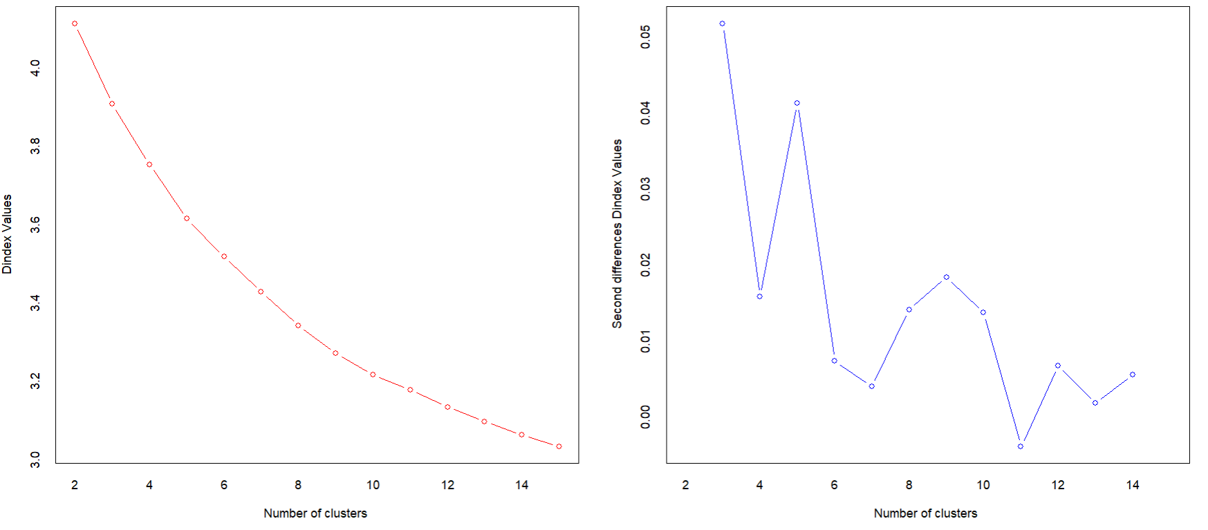
result <- NbClust(data = x, min.nc=2, max.nc = 15, method = 'ward.D')
result
> result <- NbClust(data = x, min.nc=2, max.nc = 15, method = 'ward.D')
*** : The Hubert index is a graphical method of determining the number of clusters.
                In the plot of Hubert index, we seek a significant knee that corresponds to a
                significant increase of the value of the measure i.e the significant peak in Hubert
                index second differences plot.

*** : The D index is a graphical method of determining the number of clusters.
                In the plot of D index, we seek a significant knee (the significant peak in Dindex
                second differences plot) that corresponds to a significant increase of the value of
                the measure.

*******************************************************************
* Among all indices:
* 7 proposed 2 as the best number of clusters
* 7 proposed 3 as the best number of clusters
* 2 proposed 5 as the best number of clusters
* 1 proposed 10 as the best number of clusters
* 2 proposed 11 as the best number of clusters
* 1 proposed 14 as the best number of clusters

                   ***** Conclusion *****

* According to the majority rule, the best number of clusters is  2


******************************************************************* 
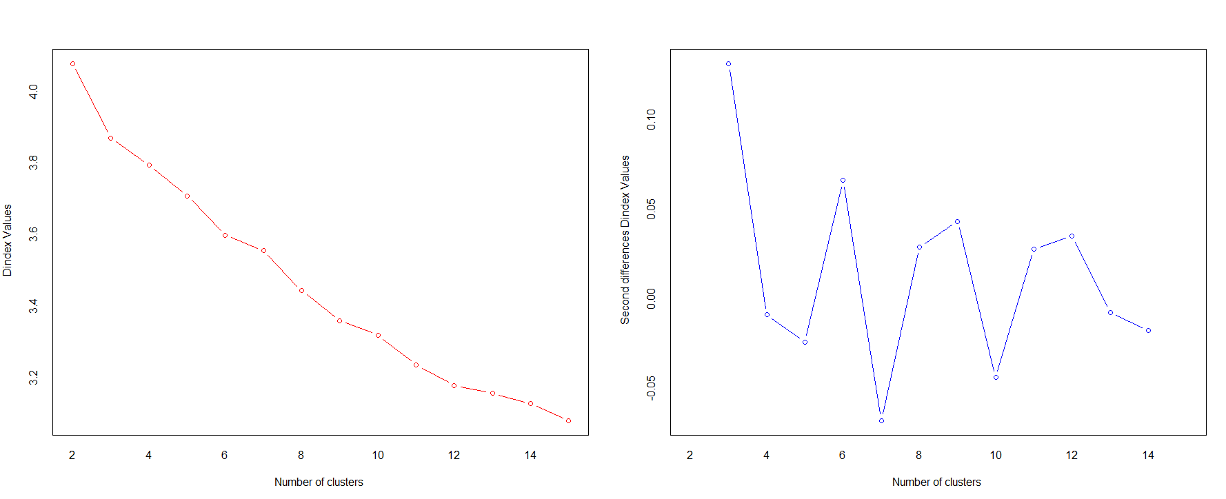
result <- NbClust(data = x, min.nc=2, max.nc = 15, method = 'ward.D2')
result
> result <- NbClust(data = x, min.nc=2, max.nc = 15, method = 'ward.D2')
*** : The Hubert index is a graphical method of determining the number of clusters.
                In the plot of Hubert index, we seek a significant knee that corresponds to a
                significant increase of the value of the measure i.e the significant peak in Hubert
                index second differences plot.

*** : The D index is a graphical method of determining the number of clusters.
                In the plot of D index, we seek a significant knee (the significant peak in Dindex
                second differences plot) that corresponds to a significant increase of the value of
                the measure.

*******************************************************************
* Among all indices:
* 9 proposed 2 as the best number of clusters
* 6 proposed 3 as the best number of clusters
* 1 proposed 5 as the best number of clusters
* 2 proposed 7 as the best number of clusters
* 1 proposed 12 as the best number of clusters
* 1 proposed 13 as the best number of clusters

                   ***** Conclusion *****

* According to the majority rule, the best number of clusters is  2


******************************************************************* 
# 비계층적 군집분석
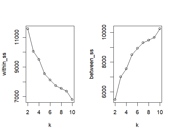
withss <- c() ; betss <- c()
for (i in 2:10) {
set.seed(0)
m2 <- kmeans(x, i)
withss <- c(withss, m2$tot.withinss)
betss <- c(betss, m2$betweenss)
}
par(mfrow = c(1,2))
plot(2:10, withss, xlab = 'k',
ylab = 'within_ss', type = 'o')
plot(2:10, betss, xlab = 'k',
ylab = 'between_ss', type = 'o')
set.seed(0)
m2 <- kmeans(x, 2)
> m2
K-means clustering with 2 clusters of sizes 375, 194

Cluster means:
  radius_mean texture_mean perimeter_mean  area_mean
1  -0.4825702   -0.2388313     -0.4999790 -0.4777212
2   0.9328033    0.4616584      0.9664542  0.9234301
  smoothness_mean compactness_mean concavity_mean
1      -0.3107301       -0.5255563     -0.5785267
2       0.6006381        1.0158949      1.1182861
  concave_points_mean symmetry_mean fractal_dimension_mean
1           -0.586655    -0.3088121             -0.1490098
2            1.133998     0.5969307              0.2880344
   radius_se  texture_se perimeter_se    area_se smoothness_se
1 -0.4276089 -0.02109138   -0.4305928 -0.4013983   -0.02381032
2  0.8265636  0.04076942    0.8323315  0.7758988    0.04602510
  compactness_se concavity_se concave_points_se symmetry_se
1     -0.3698751   -0.3343034        -0.3973627  -0.0748643
2      0.7149647    0.6462051         0.7680980   0.1447119
  fractal_dimension_se radius_worst texture_worst perimeter_worst
1           -0.2366141   -0.5173986    -0.2512569      -0.5318435
2            0.4573726    1.0001262     0.4856771       1.0280479
  area_worst smoothness_worst compactness_worst concavity_worst
1 -0.4989187       -0.3158003        -0.4918085      -0.5363714
2  0.9644047        0.6104387         0.9506607       1.0368003
  concave_points_worst symmetry_worst fractal_dimension_worst
1            -0.579591     -0.3030883              -0.3364329
2             1.120343      0.5858665               0.6503213

Clustering vector:
  [1] 2 2 2 2 2 2 2 2 2 2 1 2 2 1 2 2 1 2 2 1 1 1 2 2 2 2 2 2 2 2
 [31] 2 2 2 2 2 2 2 1 1 1 1 1 2 2 1 2 1 2 1 1 1 1 1 2 1 1 2 2 1 1
 [61] 1 1 2 1 2 2 1 1 2 1 2 1 2 1 1 2 1 2 2 1 1 2 2 2 1 2 1 2 1 2
 [91] 1 1 1 1 2 2 1 1 1 1 1 1 1 1 1 2 1 1 2 1 1 1 2 1 1 1 1 2 2 1
[121] 1 2 2 1 1 1 1 2 2 2 1 2 2 1 2 1 1 1 2 1 1 2 1 1 1 1 2 1 1 1
[151] 1 1 2 1 1 1 2 1 1 1 1 2 2 1 2 1 1 2 2 1 1 1 2 1 1 1 2 2 1 1
[181] 2 2 1 1 1 1 1 1 1 1 2 1 1 2 2 1 2 2 2 2 1 2 2 2 1 1 1 1 1 1
[211] 2 1 2 2 2 2 1 1 2 2 1 1 1 2 1 1 1 1 1 2 2 1 1 2 1 1 2 2 1 2
[241] 1 1 2 1 2 1 1 2 1 1 2 1 2 2 2 1 2 2 2 2 2 1 2 1 2 2 1 1 1 1
[271] 1 1 2 1 1 1 1 1 1 1 2 1 2 2 1 1 1 1 1 1 2 1 1 1 1 1 1 1 1 1
[301] 2 1 2 1 1 1 1 1 1 1 1 1 1 1 1 1 1 2 2 1 1 2 1 2 1 1 1 1 2 2
[331] 2 1 1 1 1 2 1 2 1 2 1 1 1 2 1 1 1 1 1 1 1 2 2 2 1 1 1 1 1 1
[361] 1 1 1 1 1 2 2 1 2 2 2 1 2 2 1 1 2 1 1 2 1 1 1 1 1 1 1 1 1 2
[391] 1 1 2 2 1 1 1 1 1 1 2 1 1 1 1 1 1 1 2 1 1 1 1 1 1 1 1 2 1 1
[421] 1 2 1 1 1 1 1 1 1 1 2 1 2 2 1 1 1 1 1 1 1 2 1 1 1 1 2 1 1 2
[451] 1 2 1 1 1 1 1 1 1 1 2 2 1 1 1 2 1 1 2 1 1 1 1 1 1 1 1 1 1 2
[481] 1 1 1 1 1 2 1 2 1 1 1 1 2 1 1 1 1 1 2 2 1 2 1 2 2 2 1 1 1 2
[511] 1 1 2 1 1 1 2 2 1 1 1 2 1 1 1 1 1 1 1 1 1 1 1 2 1 2 1 1 1 1
[541] 1 2 1 1 1 1 1 1 1 1 1 1 1 1 1 1 1 1 1 1 1 1 2 2 2 2 2 2 1

Within cluster sum of squares by cluster:
[1] 4971.437 6603.711
 (between_SS / total_SS =  32.1 %)

Available components:

[1] "cluster"      "centers"      "totss"        "withinss"
[5] "tot.withinss" "betweenss"    "size"         "iter"
[9] "ifault"
# 군집은 2개 (샘플사이즈는 각 375, 194)
# between_ss / total_ss = 32.1%
m2 <- kmeans(x, 3)
m2
> m2
K-means clustering with 3 clusters of sizes 110, 100, 359

Cluster means:
  radius_mean texture_mean perimeter_mean  area_mean
1   1.6176587    0.6260620      1.6225732  1.6616915
2  -0.1721774    0.1788294     -0.1006558 -0.2198210
3  -0.4477011   -0.2416428     -0.4691295 -0.4479219
  smoothness_mean compactness_mean concavity_mean
1       0.3982143        0.9297963      1.2382477
2       0.8484791        1.0345212      0.7803190
3      -0.3583607       -0.5730633     -0.5967664
  concave_points_mean symmetry_mean fractal_dimension_mean
1           1.4856628     0.4317906             -0.2866671
2           0.4989880     0.7521312              1.1829407
3          -0.5942109    -0.3418108             -0.2416732
    radius_se  texture_se perimeter_se    area_se smoothness_se
1  1.44001760  0.09373762   1.40414509  1.4222534   -0.07260779
2 -0.08495483  0.02338187  -0.01781494 -0.1722055    0.43926501
3 -0.41756672 -0.03523489  -0.42527706 -0.3878199   -0.10011043
  compactness_se concavity_se concave_points_se symmetry_se
1      0.4786511    0.4393663         0.7871419  0.05437929
2      1.0737418    0.8897247         0.7514795  0.28620432
3     -0.4457543   -0.3824590        -0.4505113 -0.09638483
  fractal_dimension_se radius_worst texture_worst perimeter_worst
1            0.1189330   1.66528388     0.5424224     1.655385195
2            1.0255153  -0.08815198     0.3111937    -0.007008775
3           -0.3221007  -0.48569924    -0.2528853    -0.505268785
  area_worst smoothness_worst compactness_worst concavity_worst
1  1.6834662        0.3365925         0.6697022       0.8858320
2 -0.1563397        0.9682984         1.1787346       1.0441360
3 -0.4722766       -0.3728552        -0.5335395      -0.5622705
  concave_points_worst symmetry_worst fractal_dimension_worst
1             1.272063      0.3000824              0.08399194
2             0.742345      0.8092044              1.38339588
3            -0.596550     -0.3173524             -0.41108273

Clustering vector:
  [1] 1 1 1 2 1 2 1 2 2 2 3 2 1 3 2 2 3 2 1 3 3 3 2 1 1 1 2 1 2 1
 [31] 1 2 1 1 2 2 2 3 3 2 3 2 1 2 3 1 3 2 3 3 3 3 3 1 3 3 1 2 3 3
 [61] 3 3 2 3 2 2 3 3 2 3 1 2 2 3 3 1 3 1 1 3 3 2 1 1 3 1 3 1 3 2
 [91] 3 3 3 3 2 1 3 3 3 2 3 3 3 3 3 2 3 3 1 3 3 2 2 3 3 3 3 2 2 3
[121] 3 1 1 3 3 3 3 1 2 1 3 3 3 3 1 3 3 3 1 3 3 3 3 3 3 2 2 3 3 3
[151] 3 2 2 3 3 3 1 3 3 3 3 1 1 3 1 3 3 3 1 3 3 3 2 3 3 3 2 2 3 3
[181] 1 1 3 3 3 3 3 3 3 3 2 3 3 2 2 3 2 1 1 2 3 1 1 2 3 3 3 3 2 3
[211] 1 3 1 2 2 2 2 3 1 1 3 3 3 2 3 3 3 3 3 2 2 3 3 1 3 3 1 1 3 1
[241] 3 3 2 3 1 3 3 2 3 3 1 3 1 3 1 3 1 2 1 2 1 3 1 3 1 1 3 3 3 2
[271] 3 3 1 3 3 3 3 3 3 3 1 3 1 2 3 3 3 3 2 3 2 3 3 3 3 3 3 3 3 3
[301] 1 3 1 3 3 3 3 3 3 3 3 3 3 3 3 3 3 1 2 3 3 1 3 1 3 3 3 3 2 2
[331] 2 3 3 3 3 1 3 1 3 1 3 3 3 1 3 3 3 3 3 3 3 2 1 2 3 3 2 3 3 3
[361] 3 3 3 3 3 1 1 3 1 1 2 3 1 1 3 3 2 3 3 2 3 3 3 2 3 3 3 3 2 1
[391] 3 3 2 1 3 3 3 3 3 3 2 3 3 3 3 3 3 3 1 3 3 3 3 3 3 3 3 1 3 3
[421] 3 2 3 3 3 3 3 3 3 3 2 3 1 1 3 2 3 3 3 3 2 1 3 3 3 3 1 3 3 1
[451] 3 1 3 3 3 3 3 3 3 3 1 1 3 3 3 2 3 3 1 2 3 3 3 3 3 3 3 3 3 2
[481] 3 3 3 3 3 2 3 1 3 3 3 3 1 3 3 3 2 3 1 1 3 2 3 1 2 2 3 2 3 2
[511] 3 3 2 3 3 3 1 1 3 3 2 1 3 3 3 3 3 3 3 3 3 3 3 1 3 1 3 2 3 2
[541] 3 2 3 3 3 3 3 3 3 3 3 3 3 3 3 3 3 3 3 3 3 3 2 1 1 1 3 1 3

Within cluster sum of squares by cluster:
[1] 2894.489 2791.854 4357.771
 (between_SS / total_SS =  41.1 %)

Available components:

[1] "cluster"      "centers"      "totss"        "withinss"
[5] "tot.withinss" "betweenss"    "size"         "iter"
[9] "ifault"
# 군집은 3개 (샘플사이즈는 각 110, 100, 359)
# between_ss / total_ss = 41.1%
[ 문제풀이 ]
# STEP1: 데이터 로딩)
cancer <- read.csv('cancer.csv')
cancer$diagnosis <- factor(cancer$diagnosis)
# STEP2: 불필요 변수 제거)
cancer$id <- NULL
# STEP3: 스케일링
cancer[,-1] <- scale(cancer[,-1])
# STEP4: 계층적 군집분석 수행)
X <- cancer[,-1]
d1 <- dist(X)
# 학습
m1 <- hclust(d1, method = 'single') # 최단거리법
m2 <- hclust(d1, method = 'complete') # 최장거리법
m3 <- hclust(d1, method = 'centroid') # 중심연결법
m4 <- hclust(d1, method = 'average') # 평균연결법
m5 <- hclust(d1, method = 'ward.D') # 와드1
m6 <- hclust(d1, method = 'ward.D2') # 와드2
# 시각화
dev.new()
par(mfrow=c(2,3))
plot(m1, hang = -1, main = 'Single')
rect.hclust(m1, k = 2)
plot(m2, hang = -1, main = 'Complete')
rect.hclust(m2, k = 2)
plot(m3, hang = -1, main = 'Centroid')
rect.hclust(m3, k = 2)
plot(m4, hang = -1, main = 'Average')
rect.hclust(m4, k = 2)
plot(m5, hang = -1, main = 'Ward.D')
rect.hclust(m5, k = 2)
plot(m6, hang = -1, main = 'Ward.D2')
rect.hclust(m6, k = 2)
# 평가
library(NbClust)
result <- NbClust(data = X, # 데이터
min.nc = 2, # 최소군집수
max.nc = 10, # 최대군집수
method = 'ward.D') # 군집간 거리
result
# *******************************************************************
# * Among all indices:
# * 8 proposed 2 as the best number of clusters
# * 7 proposed 3 as the best number of clusters
# * 2 proposed 5 as the best number of clusters
# * 1 proposed 7 as the best number of clusters
# * 2 proposed 10 as the best number of clusters
#
# ***** Conclusion *****
#
# * According to the majority rule, the best number of clusters is 2
# STEP4: 비계층적 군집분석 수행)
set.seed(0)
m1 <- kmeans(X, 2)
m1
'아이티윌_데이터 분석 55기 > 문제풀이_통계 및 분석' 카테고리의 다른 글
| #16-2. 16일차 퀴즈에 대한 문제풀이 (0) | 2026.05.07 |
|---|---|
| #15-2. 15일차 퀴즈에 대한 문제풀이 (0) | 2026.05.06 |
| #11-2. 11일차 퀴즈에 대한 문제풀이 (0) | 2026.04.27 |
| #7-2. 7일차 퀴즈에 대한 문제풀이 (0) | 2026.04.21 |
| #5-2. 5일차 퀴즈에 대한 문제풀이 (0) | 2026.04.17 |